Chapter 6 Conditionals, Control Flow, and Functions
Welcome to Lesson 6. In this lesson, you will write conditional statements, create loops, design functions, handle predictable errors, and apply functions across data structures.
Lesson 6 Outline
- Writing conditional statements
- Creating loops
- User-defined functions
- The apply family of functions
1. Writing conditional statements
Early on, we learned about different types of comparison and logical operators. For example, comparison operators include <, <=,== and so on. These operators return a Boolean value, TRUE or FALSE.
Let’s do a quick review of comparison operators.
## [1] FALSE## [1] FALSE FALSE FALSE FALSE TRUE## [1] FALSE FALSE TRUE FALSE FALSEThere are also a set of logical operators that include:
!&|
& and | compare values element by element and return a logical vector. && and || examine only the first value of each side and stop as soon as the result is known. Use & and | for vectorized data operations; use && and || for single conditions in control-flow statements such as if.
Let’s do a quick review of logical operators.
Ex. 1
We assign legal to the Boolean value TRUE and then use the logical not (!) operator to negate the variable legal which returns the value of FALSE.
## [1] FALSEEx. 2
We assign customer to the Boolean value TRUE and over50 to the value FALSE. Then we use the logical and (&) operator to evaluate both variables. If both are TRUE, then result returned is TRUE. If one or none of the values are TRUE, then the result is FALSE.
## [1] FALSEEx. 3
Just in the previous example, we assign customer to the Boolean value TRUE and over50 to the value FALSE. Then we use the logical or (|) operator to evaluate both variables. If both are TRUE, then result returned is TRUE. If one is TRUE, then result returned is TRUE. If neither of the values are TRUE, then the result is FALSE.
## [1] TRUEConditional statements
A conditional statement evaluates a condition to see if it is TRUE. Conditional statements may make use of comparative and logical operators.
A type of conditional statement used to evaluate if a condition is TRUE is called an if statement.
Let’s look at an example of the structure of an if statement:
The if is followed by a set of parentheses and inside is the condition being evaluated for truth. If it is true, then we may specify an action such as update a variable. If the condition is FALSE no action occurs.
if (condition) {
  # do something when the condition is TRUE
}
Ex 1.
Let’s construct a real example that evaluates the value assigned to a variable price. The condition is price < 10. This condition will evaluate to FALSE. Therefore nothing is printed.
Ex 2.
Let’s change Ex.1. We’ll change the value of price to 9.99. In this case, This is an excellent deal will be printed to the screen. In other words, the code between the opening and closing curly brackets will run.
## [1] "This is an excellent deal!"Conditional statements using if/else logic
You can add on an else onto an if statement. If the test condition is not met, that is, it evaluates to FALSE, the else code will run.
The basic structure is:
Ex 3.
Let’s build on Ex. 1 where price is set to 15.99 and add an else statement. You’ll notice that the print statement following the if is ignored and the print statement within the else clause has run.
price <- 15.99

if (price < 10) {
  print("This is an excellent deal!")

} else {
print("This product is too expensive")
}## [1] "This product is too expensive"Take note of the curly brackets in this example. The placement is important. The if and else both have an opening and closing brace. The else statement must appear on the same line as the closing if curly bracket.
Nested if...else if statements
An if...else if...else chain selects one block of code from more than two alternatives. R evaluates the conditions from top to bottom and runs the first matching branch.
The syntax of if...else if statement is:
if ( test_expression1) {
statement1
} else if ( test_expression2) {
statement2
} else if ( test_expression3) {
statement3
} else {
statement4
}
Ex. 4
Let’s modify Ex. 3
price <- 15.99

if (price < 10) {
  print("This is an excellent deal!")
} else if (price < 11) {
  print("This is a fair price!")
} else if (price < 12) {
  print("This product is slightly overpriced")
} else {
  print("This product is overpriced")
}
Try it
Test your program out by changing the value of price to ensure it evaluates the condition as you have planned.
R ifelse() function
ifelse() is a vectorized conditional function. It evaluates a logical vector and selects an element from yes or no for each position. Use ordinary if...else for scalar control flow and ifelse() when producing a vector of results.
Syntax of ifelse() function
Here, test is a logical vector. Each output element comes from yes when the corresponding condition is TRUE and from no when it is FALSE.
Ex. 5
In the example below, the ifelse() function evaluates the vector FALSE FALSE TRUE FALSE that resulted from the expression:a %% 2 == 0
## [1] "odd" "odd" "even" "odd"Ex. 6
Let’s say you want to evaluate a vector for NA values and print output to the screen based on whether there is an NA value or not. We can use the ifelse() function along with the is.na() function.
## [1] "NA" "Not NA" "Not NA" "Not NA"2. Creating loops
Loops repeat a block of code. This lesson introduces two common control structures in R: while and for loops.
The while loop is used when you want to execute some code some number (possibly an unknown number) of times.
Syntax of while loop
Here, test_expression is evaluated and the body of the loop is entered if the result is TRUE.
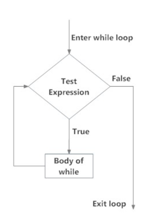
Figure 6.1: Structure of a while loop
The statements inside the loop are executed and the flow returns to evaluate the test_expression again.
This is repeated each time until test_expression evaluates to FALSE, in which case, the loop exits.
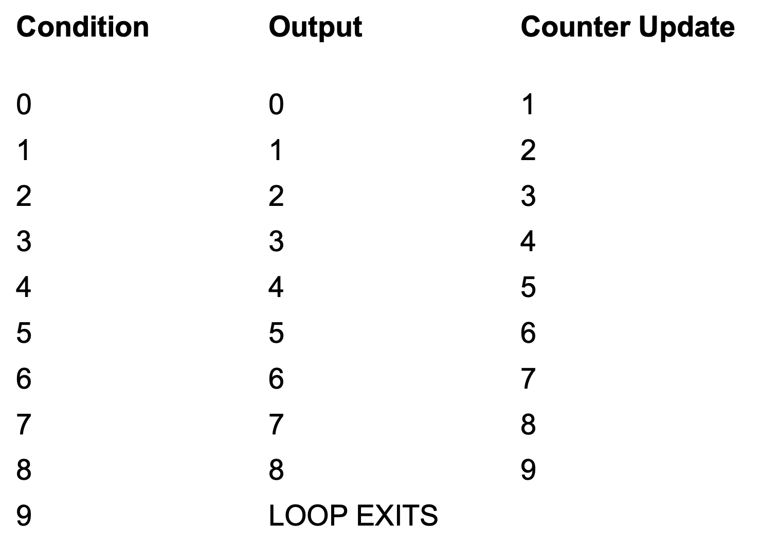
Figure 6.2: Flow of a while loop
Let’s look at a few examples:
Ex. 1
In the example below, how many times with the loop iterate?
Run the code to see it for yourself. Before running any while loop, identify the statement that will eventually make its condition FALSE. To interrupt a runaway computation in RStudio, press Esc on macOS or click the Stop button in the Console pane.
You’ll note that the loop will iterate ten times. First, when x is initialized to 10 and thereafter we decrease x by 1, until x = 0 where x > 0 finally evaluates to FALSE.
Ex. 2
In the example below, counter is initialized to zero. The test expression in the while statement evaluates to see counter is less than 9, prints the value of counter and then increments it by 1.
How many times will this loop iterate?
## [1] 0
## [1] 1
## [1] 2
## [1] 3
## [1] 4
## [1] 5
## [1] 6
## [1] 7
## [1] 8
The loop will iterate 9 times, printing the sequence 0 through 8.
What if we change test condition to while(counter > 9)? How many times would the loop iterate?
This creates an infinite loop because counter begins above 9 and increases on every iteration. Interrupt it with Esc or RStudio’s Stop button; you do not need to restart or power down the computer.
It is important to examine the relationship between the test expression and the control, which in this case in the counter.
Here, counter > 9 remains TRUE because the loop increases counter. Changing the update to counter <- counter - 1 would make the condition FALSE after one iteration.
The for loop
Another type of loop used in R is called a for loop.
A for loop is used to iterate over a vector, such as a column in a data frame.
The syntax is as follows:
Here, sequence is a vector and value takes on each of one of the values in the sequence. During each iteration, statement is evaluated.
A for loop visits each element of a supplied sequence, so the sequence determines the number of iterations.
In the code below, the iterator (in this case, i) takes on the values in the vector c(1,2,3,4) sequentially through each “loop” of the code that is between the brackets—in this case, print(i).
## [1] 1
## [1] 2
## [1] 3
## [1] 4
Loops and conditional statements using if/else logic
Let’s build a program that counts prices below $10.
You can approach it the following way:
First create the price vector and initialize num_cheap to zero. Then loop through the prices. Whenever a price is below 10, increment the counter. After the loop exits, print the result.
prices <- c(12.43, 9.99, 18.22, 7.25, 0.50)
num_cheap <- 0
for (p in prices) {
    if (p < 10) {
        num_cheap <- num_cheap + 1
    }
}
print(num_cheap)
## [1] 33. User-Defined Functions
Functions package a reusable set of instructions behind a meaningful name. They can accept inputs called arguments and return a result.
Some functions are built in such as:
toupper
## [1] "HELLO WORLD"mean
## [1] 3is.numeric
## [1] TRUEis.na
## [1] TRUEsqrt
## [1] 5Functions operate on arguments and usually return a value. For example, sqrt(25) receives 25 and returns 5. In R, the final evaluated expression is returned automatically; use return() when an early or explicit return improves clarity.
In addition to using pre-existing functions from R packages, we can write our own.
- Functions are useful for executing repetitive commands.
- Planning is key to writing effective functions.
This example separates a function definition from a function call.
Part 1 — define the function:
Part 2 — call the function:
## [1] "The value 34 is returned"Let’s apply this structure to a short problem.
Suppose we want to have a function to act on our data that adds 2 to every value. How would we design this function?
Function Pseudocode
We begin by drafting out the main components of a function.
First, let’s give our function a name. We’ll call it add_two.
Next, assign a function definition created with function() to that name. Place the parameter inside parentheses and the function body inside braces. Here the parameter is called my_parameter.
Now let’s set up our function call.
The empty function is valid, but calling it returns NULL because its body does not compute a value. Add an expression that uses the parameter.
In this case, we are just adding 2 to my parameter.
Now, when we call add_two and pass in a number, we see a value is returned which is my_parameter + 2.
## [1] 24What happens when we don’t pass in a numeric value?
The error is: Error in my_parameter + 2 : non-numeric argument to binary operator
Can you see why this error was given? You’ll notice that the string hello caused this error.
How can we plan for user error?
Validate the input with is.numeric(). If it is not numeric, call stop() with an informative error; otherwise return the computed result.
add_two <- function(my_parameter) {
  if (!is.numeric(my_parameter)) {
    stop("my_parameter must be numeric.")
  }
  my_parameter + 2
}
Calling the function with text produces the deliberate validation error. Keep this demonstration unevaluated so the book continues rendering:
Let’s try calling add_two again with a numeric value. You can see the function works as it should when a numeric value is provided.
## [1] 5Pass in multiple arguments
Let’s create a function that takes more than one argument. We’ll call this function add_together and include 2 parameters or arguments in the function declaration.
add_together <- function(x, y) {
  if (!is.numeric(x) || !is.numeric(y)) {
    stop("x and y must both be numeric.")
  }
  x + y
}
Now, let’s call the function, add_together.
## [1] 20Let’s call it, yet again, but this time passing in a number and as string.
Alternative function call, with literal specification
## [1] 15Try it. Write a function that averages two numbers
This can be easily achieved by modifying the add_together function and changing the computation to (x + y)/2.
average_two <- function(x, y) {
  if (!is.numeric(x) || !is.numeric(y)) {
    stop("x and y must both be numeric.")
  }
  (x + y) / 2
}

average_two(1, 2)
## [1] 1.5average_two() returns a result when both arguments are numeric and raises the deliberate validation error when either supplied value is nonnumeric. If an argument is omitted entirely, R instead reports that the required argument is missing:
Error in average_two(1) : argument "y" is missing, with no default
That default message is accurate but may not explain how a user should correct the call. Good function design anticipates common input problems and reports actionable errors.
Use missing() at the beginning of a function when you want to provide a custom message for omitted required arguments:
add_together <- function(x, y) {
  if (missing(x) || missing(y)) {
    stop("Provide both x and y.")
  }
  if (!is.numeric(x) || !is.numeric(y)) {
    stop("x and y must both be numeric.")
  }
  x + y
}
Adding a tryCatch() block
Use tryCatch() when a function can recover from an anticipated error or convert it into a controlled result. The protected expression goes first, followed by handlers such as error = function(e).
safe_add <- function(x, y) {
  tryCatch({
    if (missing(x) || missing(y)) {
      stop("Provide both x and y.")
    }
    if (!is.numeric(x) || !is.numeric(y)) {
      stop("x and y must both be numeric.")
    }
    x + y
  }, error = function(e) {
    paste("Error:", conditionMessage(e))
  })
}

safe_add(3)
## [1] "Error: Provide both x and y."## [1] "Error: x and y must both be numeric."## [1] 8An undefined object supplied as an argument—for example, safe_add(not_defined, 3)—fails while R evaluates the function call, before execution enters safe_add(). An internal tryCatch() therefore cannot catch that particular error. Use a quoted test value when demonstrating input validation.
4. Apply family of functions
The apply family runs a function across elements or data components without writing an explicit loop. Two useful members are:
lapply(X, FUN), which always returns a list.sapply(X, FUN), which callslapply()and then attempts to simplify the result to a vector or matrix.
For a data frame, each column is an element. The following code finds the maximum of each column:
quarterly_metrics <- data.frame(
  revenue = c(120, 135, 142, 151),
  orders = c(48, 52, 55, 61)
)

sapply(quarterly_metrics, max)
## revenue orders
## 151 61Use lapply() when you want a predictable list result:
## $revenue
## [1] 151
##
## $orders
## [1] 61
You can also supply your own function. This function calculates a mean while ignoring missing values:
##     rating complaints privileges   learning     raises   critical    advance
##   64.63333   66.60000   53.13333   56.36667   64.63333   74.76667   42.93333
Check the result against R’s summary:
##      rating        complaints     privileges       learning         raises
##  Min.   :40.00   Min.   :37.0   Min.   :30.00   Min.   :34.00   Min.   :43.00
##  1st Qu.:58.75   1st Qu.:58.5   1st Qu.:45.00   1st Qu.:47.00   1st Qu.:58.25
##  Median :65.50   Median :65.0   Median :51.50   Median :56.50   Median :63.50
##  Mean   :64.63   Mean   :66.6   Mean   :53.13   Mean   :56.37   Mean   :64.63
##  3rd Qu.:71.75   3rd Qu.:77.0   3rd Qu.:62.50   3rd Qu.:66.75   3rd Qu.:71.00
##  Max.   :85.00   Max.   :90.0   Max.   :83.00   Max.   :75.00   Max.   :88.00
##     critical        advance
##  Min.   :49.00   Min.   :25.00
##  1st Qu.:69.25   1st Qu.:35.00
##  Median :77.50   Median :41.00
##  Mean   :74.77   Mean   :42.93
##  3rd Qu.:80.00   3rd Qu.:47.75
##  Max.   :92.00   Max.   :72.00
6.1 Exercise 6.1
Write a function called describe_variable(x) that returns a named vector containing the mean, median, minimum, and maximum. Each calculation should ignore missing values. Apply the function to every column of the built-in attitude data frame with sapply(), and inspect the resulting matrix.
6.2 Exercise 6.2
Import the Airbnb dataset from https://becomingvisual.com/rfundamentals/airbnb.csv.
Write a function called
check_for_na(x)that returns the number of missing values inx. Apply it to every column of the Airbnb data and report the result.Using a
forloop and anifstatement, count listings whoseneighbourhoodis either"Greenwich Village"or"West Village". Compare your loop result with a vectorized calculation using%in%.
6.3 Assignment 6a
Import the Airbnb dataset from https://becomingvisual.com/rfundamentals/airbnb.csv.
Write a function that accepts the Airbnb data frame and returns the average number of reviews and average price for each neighborhood. Ignore missing values explicitly.
Extend the function so it groups by both room type and neighborhood and returns the same two metrics.
Use dplyr::group_by() and dplyr::summarise(). The current reference guide is available through Posit’s dplyr cheatsheet.
6.4 Assignment 6b
Create an R Markdown document that completes the following tasks. Keep package installation commands out of the document; install any required package separately from the RStudio Console.
Create a data frame with the columns
Card_Number,Cardholder_Name,Credit_Limit, andBalance. Populate it with at least three rows of sample data. Treat card numbers as character identifiers rather than quantities.Write
check_balance(card_number, cards). It should validate its arguments and return the current balance for exactly one matching card. Handle and test at least six error conditions, including missing arguments, missing required columns, an invalid card-number type or length, a card that is not found, duplicate card numbers, and a missing or nonnumeric balance.Write
update_balance(card_number, amount, cards). It should validate the card number and amount, update exactly one matching balance, and return the updated data frame. Do not rely on or modify a hidden global data frame. Test at least six error conditions as well as a successful update.Use a
forloop to print each cardholder’s name and balance.Use
sapply()to find the largest numeric value in each applicable numeric column. Do not applymax()to identifier or name columns.
Use conditional statements for validation and tryCatch() only where the function can meaningfully handle or translate an anticipated error. Show all tests and briefly state the expected result of each one.