Chapter 2 Data Structures

Welcome to Lesson 2. You will create variables, distinguish common data types, work with vectors and data frames, represent categorical data with factors, sort values, and recognize special values used for missing or undefined data. The exercises combine short-answer questions with hands-on R coding.

Lesson 2 outline

Creating variables
Numeric, character and logical data
Vectors
Data frames
Factors
Sorting numeric, character, and factor vectors
Special values
Summary

Watch introductory video

Watch the introductory video

1. Creating variables.

One of the most important things to be able to do in any programming language is store information in variables.

You can think of variables as a label for one or more pieces of information.

When doing statistical analysis in R, all of your data (the variables you measured in your study) will be stored as variables in R. You can create variables for other things too, which we will learn later on in the course.

Variable assignment

In Lesson 1, we created the variables temperature and thermostat. In this course, use the conventional R assignment operator <-.

temperature <- 50
thermostat <- 65

Read temperature <- 90 as “assign the value 90 to temperature.” R also permits = in many assignment contexts and supports the right-assignment operator ->, but <- is the clearest and most common convention in R scripts.

temperature <- 90
thermostat <- 50

Let’s return to our temperature and thermostat example. When we type

temperature <- 50

R doesn’t return any output. It just provides you with another command prompt. However, behind the scenes, R has created a variable called temperature and given it a value of 50. You can check that this has happened by asking R to print the variable on the screen. To do this, type the name of the variable and press enter.

temperature

## [1] 50

You can also do this using the print( ) function and passing the variable as a parameter to the function.

print(temperature)

## [1] 50

Doing calculations with variables

Just as you performed calculations in lesson 1 with numbers, you can do the same with variables that contain references to numbers.

Try the example below. In this example, for a single product, we’ve created two variables cost and price and assigned them values. We then computed profit by taking the difference of price and cost and assigned the result to the variable profit. Then we printed out the result of profit.

cost <- 9.60
price <- 12
profit <- price - cost
profit

## [1] 2.4

Now, let’s assume you sold 82,342 units. Let’s compute your profit.

units <- 82342
units * profit

## [1] 197620.8

Rules and conventions for naming variables

The variables we’ve created and used in this lesson are just English-language words written using lowercase letters. However, R allows for a lot more flexibility when it comes to naming your variables.

Here’s a quick list of rules:

Variable names can be uppercase, lowercase, or mixed case alphabetic characters A-Z or a-z. Variable names can contain numeric characters 0-9, a period ., or underscore _ characters.
Variable names can only begin with a letter or period. A variable name cannot begin with a number. Avoid beginning variables with a period as a matter of convention.
Variable names cannot include spaces. Sales total = 53231 is invalid. However, sales_total and sales.total are valid variable names.
Variable names are case sensitive. SalesTotal is different from Salestotal.
Variable names cannot be one of R’s reserved words. These include: if, else, repeat, while, function, for, in, next, break, TRUE, FALSE, Inf, NaN, NA, NA_integer_, NA_real_, NA_complex_, and NA_character_.

Here’s a quick list of conventions:

Use informative variable names. Avoid names such as var1 and var2. As a general rule, using meaningful names like temperature, profit, and cost helps you (and others who may use or read your code) understand your code better. Sometimes we forget what variables like x and y mean.
Use short variable names. Avoid super long variable names such as this_is_the_price_for_widgets. widget_price is a sufficiently meaningful variable name.
For additional naming and formatting guidance, see the tidyverse style guide.

2. Numeric, character, and logical data

Variables can be of different types. For example, the variable temperature is of type “numeric.” This should make sense since we only want to assign numbers to temperature.

However, there are many different data types. That is, our variables can be assigned to values that contain numbers, words, a mix of letters and numbers, Boolean values, and much more.

For now, we will focus on three types of variables: logical, numeric, and character. Below, we’ve created these three different types of variables:

instock <- FALSE
inventory <- 0
productid <- "9882avcde32"

What type of variable is instock? Well, it is assigned a value of FALSE. TRUE and FALSE are reserved for Boolean or logical data types. Therefore, instock is of type logical.

We can also ask R to tell us how our variables are defined by using the class() function.

class(instock)

## [1] "logical"

What type of variable is inventory? Let’s ask R:

class(inventory)

## [1] "numeric"

Finally, what type of variable is productid?

class(productid)

## [1] "character"

To create a character data type, the value(s) assigned to the variable needs to be in double quotes, as shown below:

productid <- "9882avcde32"

Why do we need different data types?

We just learned how to create a variable of the types logical, numeric, and character. Also, we were able to check to see how R interprets our variables as different “types” using the class( ) function.

However, it may not be clear to you why we need to think about data types.

Let’s begin with numeric data. Variables that are of type “numeric” are afforded the privilege of mathematical manipulation. Think back to lesson 1 where we used R as a calculator. There, all the data we worked with was numeric. We could use functions like round(), sqrt(), and abs(). In addition, we could use arithmetic operators such as +, -, /, *, and ^.

Variables and data must be of type numeric to perform mathematical calculations.

Let’s look at a quick example:

hours_worked <- 4
hourly_rate <- 27.50
hours_worked * hourly_rate

## [1] 110

The calculation being performed is the product of 4 * 27.50, which is 110.

Let’s see another example. For the hours_worked variable, let’s put double quotes around the assigned value of 4. See below.

hours_worked <- "4"
hourly_rate <- 27.50

Now, let’s try to multiply hours_worked * hourly_rate.

hours_worked * hourly_rate

Error in hours_worked * hourly_rate : 
  non-numeric argument to binary operator

In this example, you can see from the error that R cannot perform the multiplication. Why? This is because the hours_worked variable is now of type character, not numeric. Let’s prove it.

class(hours_worked)

## [1] "character"

Shouldn’t all numbers be of type numeric?

The short answer is no. There are some numbers, such as product bar codes, years, dates, and identification numbers, that should be treated as characters or a different data type such as a factor (more on factors later on in this lesson).

What about logical data? Couldn’t we just use the character data type for true and false values?

You could store the words "true" and "false" as character values, but R would treat them as text rather than logical values. Use the unquoted constants TRUE and FALSE for logical data.

Logical values work directly with comparison and logical operators. Comparison expressions return values of type logical.

Let’s try to prove this:

status <- 4 > 1
status

## [1] TRUE

class(status)

## [1] "logical"

In the example above, we assign the variable status the returned value of the expression 4 > 1. That returned value is TRUE. The value of TRUE is now assigned to the variable status, which makes it a logical data type. In addition, you can not perform additional operations on a character data type:

!status

## [1] FALSE

stat <- "TRUE"
!stat

Error in !stat : invalid argument type

3. Vectors

A vector stores multiple values of a common atomic type. Numeric, character, and logical vectors are foundational data structures in R.

Let’s say that we are grading an assignment from a class of 12 students. The grades for the assignment are as follows

100, 0, 90, 92, 94, 94, 94, 100, 0, 90, 98, 98

How can we create a variable that can contain multiple values?

Creating a vector

To create a vector, use the combine function called c( ). Then, pass the values you want to store in the vector to the c( ) function, separated by commas. To view your vector, type in the variable name and press enter. In the example below, we have created a vector of 12 elements in which each element is a grade.

grades <- c(100, 0, 90, 92, 94, 94, 94, 100, 0, 90, 98, 98)
grades

##  [1] 100   0  90  92  94  94  94 100   0  90  98  98

Getting information out of vectors

Suppose you want to know the grade of just the first student. You would want to reference the first element in the vector.

grades[1]

## [1] 100

The number within the square brackets [ ] is the index. The index of a vector begins with the number 1. That is, grades[1] references the value of 100 in the variable grades. Aside: Most programming languages begin indexing at 0, not 1.

Think of your grade variable as a single row of data, with each element stored in its cell. To reference a particular value, you need to reference the column number (see Figure 1)

1	2	3	4	5	6	7	8	9	10	11	12
100	0	90	92	94	94	94	100	0	90	98	98

Figure 1. A visual representation of the 12 grades in R with the corresponding indices 1 -12 (in gray).

To return the second value in the vector, type

grades[2]

## [1] 0

and so on….

Altering elements in a vector

Suppose I needed to correct a few grades. Those students who received zeros on their homework have since completed their homework. Therefore, the grade list needs to be updated.

How do you update values in a vector?

There are two options. 1) recreate the entire vector, or 2) replace only those elements in the vector that need to be replaced.

Let’s go with option 2. This is more efficient. With option 1, this would require more typing.

Which elements of the vector contain zeros? Elements 2 and 9. Let’s just replace those values. We can replace values through reassignment.

grades[2] <- 80
grades[9] <- 75
grades

##  [1] 100  80  90  92  94  94  94 100  75  90  98  98

What if I wanted to curve all of the homework grades by 2 points? How could I do this without having to update every element individually or create an entirely new vector of grades?

You can add 2 points to each element in a vector the following way:

grades + 2

##  [1] 102  82  92  94  96  96  96 102  77  92 100 100

However, the values won’t be updated. For example, if you type:

grades

##  [1] 100  80  90  92  94  94  94 100  75  90  98  98

You’ll notice that the command grades+2 didn’t update. It just calculated the results but did not update the vector.

To update the vector, type

grades <- grades + 2
grades

##  [1] 102  82  92  94  96  96  96 102  77  92 100 100

Extracting multiple elements from a vector

To extract a range of values from a vector such as the 3rd element through the 11th element you could use the 3:11 shorthand, see Figure 2.

1	2	3	4	5	6	7	8	9	10	11	12
102	82	92	94	96	96	96	102	77	92	100	100

Figure 2. A visual representation of the 12 grades in R with the corresponding indices 1 through 12. The yellow region highlights the range to be returned by R using grades[3:11].

grades[3:11]

## [1]  92  94  96  96  96 102  77  92 100

To extract a few elements of a vector that are not in sequence, you can use the c( ) combine function to indicate which elements you’d like to extract.

grades[c(2, 4, 5, 6)]

## [1] 82 94 96 96

Logical indexing

Logical indexing is a powerful way to manipulate data. You can use the logical operators learned in lesson one. For example, suppose I want to see all those grades that were less than 100.

grades[grades < 100]

## [1] 82 92 94 96 96 96 77 92

Counting vector elements

What if I wanted to know how many grades I recorded? How could I count the number of elements in a vector?

You can do this using a function called length( ).

length (grades)

## [1] 12

The length function will be useful later on in the course when we want use the length of a given vector a control in our loops and conditional statements.

4. Data frames

It would be more helpful if the grades were associated with student IDs. This way I can know which grade corresponds to which student.

We can do this by creating a second vector of text data.

ids <- c("ks123", "abs21", "ts32", "hgc31", "lp22", "kp89", "ss22", "yu12", "re89", "wv342", "pl32", "jgg32")
ids

##  [1] "ks123" "abs21" "ts32"  "hgc31" "lp22"  "kp89"  "ss22"  "yu12"  "re89" 
## [10] "wv342" "pl32"  "jgg32"

However, now that we have created two vectors, grades and ids, there’s no association between the two vectors. Since we created both vectors, we know that grades[1] corresponds to ids[1], but there’s no real relationship at this point. For example, if we re-ordered the data in ids to be alphabetical, ids[1] would no longer correspond to the correct value in grades[1]. This is because any time we manipulate ids, grades is unaffected. This can cause data integrity issues.

To reduce data integrity issues, it’s best if we combine the grades and IDs by using the data.frame( ) function. We want to create a list of 2 columns with ids and grades. We can do this using a different data structure called a data frame and passing our two vectors into the data.frame( ) function.

gradesheet <- data.frame(ids, grades)
gradesheet

##      ids grades
## 1  ks123    102
## 2  abs21     82
## 3   ts32     92
## 4  hgc31     94
## 5   lp22     96
## 6   kp89     96
## 7   ss22     96
## 8   yu12    102
## 9   re89     77
## 10 wv342     92
## 11  pl32    100
## 12 jgg32    100

Note that the variable gradesheet is a self-contained variable. We no longer have to refer to the vectors grades and ids. Use dim() to return the dimensions of a matrix or data frame. For gradesheet, it returns 12 rows and 2 columns. A vector does not have dimensions unless a dimension attribute has been assigned.

dim(gradesheet)

## [1] 12  2

Our data frame (gradesheet) is an independent data structure. For example, if we make changes to the grades variable in the gradesheet, it will not update the grades vector. To prove this, let’s update the first value in our grade vector (the one that we aren’t using anymore) from 102 to 0.

grades[1] <- 0
grades

##  [1]   0  82  92  94  96  96  96 102  77  92 100 100

Next, let’s see what’s stored in our gradesheet.

gradesheet

##      ids grades
## 1  ks123    102
## 2  abs21     82
## 3   ts32     92
## 4  hgc31     94
## 5   lp22     96
## 6   kp89     96
## 7   ss22     96
## 8   yu12    102
## 9   re89     77
## 10 wv342     92
## 11  pl32    100
## 12 jgg32    100

You can see that gradesheet has two columns of data: ids and grades. For the first row, list the values as ks123, 102. This proves that the grades vector is a different variable than the grades column in gradesheet. To update the gradesheet data frame, you can use the $ operator to reference a specific variable. For example, to list only the grades column from the gradesheet data frame, type

gradesheet$grades

##  [1] 102  82  92  94  96  96  96 102  77  92 100 100

Getting information out of a data frame

Our data frame called gradesheet contains two variables called grades and ids. We learned how to view the values of just grades.

gradesheet$grades

##  [1] 102  82  92  94  96  96  96 102  77  92 100 100

We use the $ operator to extract the variable you are interested in from a data frame.

Let’s say you wanted to extract a particular set of values from the grades variable in a gradesheet. For example, if you wanted to see all grades <100.

gradesheet$grades[gradesheet$grades<100]

## [1] 82 92 94 96 96 96 77 92

This statement returns all values in the grades column that are less than 100.

Information about a data frame

When you want to view the data in your data frame, you can use the View( ) function.

View(gradesheet)

This will allow you to view your data frame in a spreadsheet-like format in the upper left quadrant of RStudio; see Figure 2.1 below.

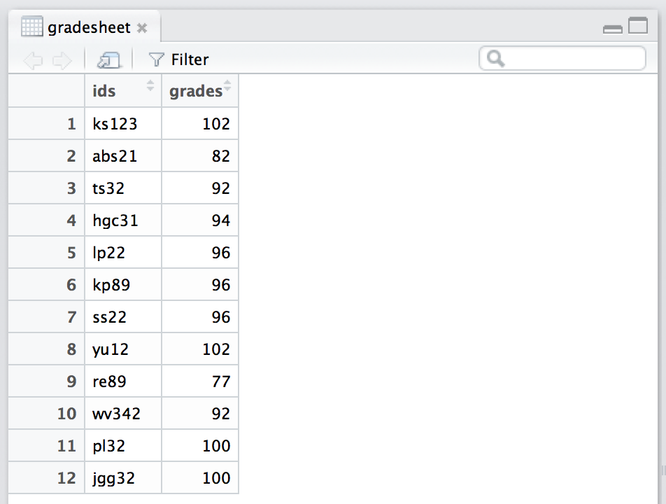
Figure 2.1: Data view using the View( ) function in RStudio.

An alternative to the View( ) function is to just type the name of the data frame as you did earlier.

gradesheet

##      ids grades
## 1  ks123    102
## 2  abs21     82
## 3   ts32     92
## 4  hgc31     94
## 5   lp22     96
## 6   kp89     96
## 7   ss22     96
## 8   yu12    102
## 9   re89     77
## 10 wv342     92
## 11  pl32    100
## 12 jgg32    100

If you wanted to know the names of the variables in your data frame without seeing the data, use the names( ) function and pass in the name of your data frame as a parameter.

names(gradesheet)

## [1] "ids"    "grades"

If you wanted to know how many columns of data you have in a data frame, you could use the length( ) function.

length(gradesheet)

## [1] 2

To know the length of a particular variable in a data frame, use the $. Notice with a variable the length function will give you the number of rows or observations.

length(gradesheet$ids)

## [1] 12

5. Factors

How do we make a distinction between nominal, ordinal, interval, and ratio scale data? How do we do this in R? There are more data types beyond the single numeric data type. Factors are the main way to represent a nominal scale variable. Nominal variables store values that have no relationship between the different possibilities (categories). For example, say you created a variable called eyes. The possible values of blue, green, hazel, etc. have no order, rank, or true zero point.

Let’s say that I have 3 teams of 4 students working together on a group project. How can I keep track of students and their groups? I might want to have a variable that keeps track of the student groups.

Let’s create a vector called groups.

groups <- c(1,1,1,1,2,2,2,2,3,3,3,3)

Next, we want to convert groups to a factor variable. This is better than having groups as a numeric variable. Numeric variables are best reserved for those values in which you’d want to perform calculations. In this case, the numbers used are just for groups. We’d never perform a calculation such as:

groups+2

##  [1] 3 3 3 3 4 4 4 4 5 5 5 5

Let’s convert groups to a factor variable so we don’t accidentally use the data in groups to perform a calculation. We can use the as.factor( ) function to convert our variable.

groups <- factor(groups)
groups

##  [1] 1 1 1 1 2 2 2 2 3 3 3 3
## Levels: 1 2 3

Notice the levels. Levels are the categories of data that are stored in our factor variable. You can see that 1, 2, or 3 are the only values stored in our vector.

Now try to add the number 2 to the groups variable.

groups + 2

## Warning in Ops.factor(groups, 2): '+' not meaningful for factors

##  [1] NA NA NA NA NA NA NA NA NA NA NA NA

R returns a warning and produces missing values because arithmetic is not meaningful for a factor. Factors represent categories, not quantities.

Factor levels

Levels refer to the range of categories represented in the groups. There are only three groups, each named 1, 2, and 3.

Let’s rename the levels from 1, 2, and 3, to group 1, group 2, and group 3. This can be done using the combine c( ) function. In the expression below, we are simply replacing 1 with group 1, 2 with group 2, and 3 with group 3. Notice that the names we used were enclosed in double quotation marks. This is necessary for factor data, especially when we use spaces.

levels(groups) <- c("group 1" , "group 2", "group 3")
levels(groups)

## [1] "group 1" "group 2" "group 3"

groups

##  [1] group 1 group 1 group 1 group 1 group 2 group 2 group 2 group 2 group 3
## [10] group 3 group 3 group 3
## Levels: group 1 group 2 group 3

Aside: The output from groups is printed on two lines in R. The first line begins with [1] and the second line begins with [10]. The 1 indicates that the line begins with the 1st element. The 10 represents the tenth element of the line you are reading.

6. Sorting numeric, character, and factor vectors

In this section, we will discuss the ways to sort a vector or data frame and combine two vectors together in a matrix and a data frame.

Sorting a numeric or character vector

A common data analysis task is to sort a variable. For numeric variables you might want to sort it in ascending or descending order. That is, you may want to sort it from the highest to the lowest values or vice-versa. For character variables, you might want to sort the data alphabetically.

You can sort variables using the sort( ) function.

The usage is: sort(x, decreasing = FALSE, ...)

TRY IT: Let’s create a simple numeric vector called datamininggrades using the c( ) function that contains the final numeric grades of sample of 10 students in their data mining course. Sort it from lowest to highest.

The grades are 90,87,69,89,58,93,99,98,76,88

datamininggrades <- c(90,87,69,89,58,93,99,98,76,88)
sort(x = datamininggrades)

##  [1] 58 69 76 87 88 89 90 93 98 99

By default, you’ll notice that R will sort a numeric vector in ascending order (from lowest to highest).

TRY IT: Sort the vector in descending order by adding a parameter for decreasing and assign it to TRUE.

sort(x = datamininggrades, decreasing = TRUE)

##  [1] 99 98 93 90 89 88 87 76 69 58

TRY IT: Next, create a simple character vector called lettergrade with the ten following values: “A-”, “B+”, “F”, “B+”, “F”, “A”, “A”, “A”, “C+”, “B+”

lettergrade <- c("A-", "B+", "F", "B+", "F", "A", "A", "A", "C+", "B+" )
sort(x=lettergrade)

##  [1] "A"  "A"  "A"  "A-" "B+" "B+" "B+" "C+" "F"  "F"

class(lettergrade)

## [1] "character"

With characters, the sort function sorts alphabetically.

Sorting a factor variable

In addition to sorting variables of type numeric and character, we can sort factor variables. Factors are sorted according to their level order. When levels have not been specified explicitly, R commonly creates them in alphabetical order.

TRY IT: To demonstrate how to sort factors, we’ll create a factor variable called lettergradefactor using the lettergrade vector we created previously. We use the factor( ) function to cast lettergrade as a factor.

lettergradefactor <- factor(lettergrade)
lettergradefactor

##  [1] A- B+ F  B+ F  A  A  A  C+ B+
## Levels: A A- B+ C+ F

Next, sort the lettergradefactor variable using the sort( ) function, just as we did earlier.

sort(lettergradefactor)

##  [1] A  A  A  A- B+ B+ B+ C+ F  F 
## Levels: A A- B+ C+ F

By default, the factor levels are alphabetically ordered. There are cases when they are not. For example, let’s return to lesson 6. If we have data that contains Likert-scale responses from Disagree to Strongly Agree, alphabetically sorting is not useful for ordinal variables. That is variables that have a clear ordering sequence.

TRY IT: Create a vector called agreement that contains the following values: “Disagree”, “Neither agree or disagree”, “Somewhat agree”, “Agree”, “Strongly Agree”.

agreement <- c("Disagree", "Neither agree or disagree", "Somewhat agree", "Agree", "Strongly Agree")
agreement

## [1] "Disagree"                  "Neither agree or disagree"
## [3] "Somewhat agree"            "Agree"                    
## [5] "Strongly Agree"

Next, convert the vector to a factor variable called agreementfactor.

agreementfactor <- factor(agreement)
agreementfactor

## [1] Disagree                  Neither agree or disagree
## [3] Somewhat agree            Agree                    
## [5] Strongly Agree           
## 5 Levels: Agree Disagree Neither agree or disagree ... Strongly Agree

Then, sort the factor variable and note how it sorts the values.

sort(agreementfactor)

## [1] Agree                     Disagree                 
## [3] Neither agree or disagree Somewhat agree           
## [5] Strongly Agree           
## 5 Levels: Agree Disagree Neither agree or disagree ... Strongly Agree

Instead, let’s define the order of the factor levels using the levels parameter of the factor function.

The usage is: factor(x = character( ), levels, labels = levels, exclude = NA, ordered = is.ordered(x))

agreementfactor <- factor(agreement, levels = c("Disagree", "Neither agree or disagree", "Somewhat agree", "Agree", "Strongly Agree"))
sort(agreementfactor)

## [1] Disagree                  Neither agree or disagree
## [3] Somewhat agree            Agree                    
## [5] Strongly Agree           
## 5 Levels: Disagree Neither agree or disagree Somewhat agree ... Strongly Agree

While it initially looked as though R was sorting factor variables alphabetically, this example proves that it sorts based on the level order.

Merging data together

It is quite common to combine several vectors into one data structure. We can either merge our data as a matrix or as a data frame.

Let’s merge the two vectors datamining grades and lettergradefactor in one data structure.

Using the cbind( ) function to create a matrix.

The cbind function essentially combines two columns into a single data structure. For future reference, there is also the rbind function used to combine rows.

For practice, let’s take the two vectors datamining grades and lettergrade factor and create a single data structure called mergegrades using the cbind function.

The usage for cbind( ) is:

cbind (vector1, vector2,…)

mergegrades <-  cbind(datamininggrades, lettergradefactor)
mergegrades

##       datamininggrades lettergradefactor
##  [1,]               90                 2
##  [2,]               87                 3
##  [3,]               69                 5
##  [4,]               89                 3
##  [5,]               58                 5
##  [6,]               93                 1
##  [7,]               99                 1
##  [8,]               98                 1
##  [9,]               76                 4
## [10,]               88                 3

What type of data structure is mergegrades?

cbind() creates a matrix, and every matrix element must have the same atomic type. Combining a numeric vector with a factor can expose the factor’s underlying integer codes, so a data frame is the safer structure for mixed types.

TRY IT: Use the data.frame( ) function to create a data frame instead of a matrix.

The usage is:

data.frame(..., row.names = NULL, check.rows = FALSE, check.names = TRUE)

finalgrades <- data.frame(datamininggrades, lettergradefactor)

As you can see below, the data.frame function preserves the native data type of each variable in the data structure.

finalgrades

##    datamininggrades lettergradefactor
## 1                90                A-
## 2                87                B+
## 3                69                 F
## 4                89                B+
## 5                58                 F
## 6                93                 A
## 7                99                 A
## 8                98                 A
## 9                76                C+
## 10               88                B+

Sorting a data frame

sort() operates on vectors, not entire data frames. To sort a data frame with base R, use order() to calculate row order.

The usage is:

with(data, expr, ...)

TRY IT: Here’s an example for you to practice that sorts a data frame.

finalgrades[order(-finalgrades$datamininggrades), ] # descending

##    datamininggrades lettergradefactor
## 7                99                 A
## 8                98                 A
## 6                93                 A
## 1                90                A-
## 4                89                B+
## 10               88                B+
## 2                87                B+
## 9                76                C+
## 3                69                 F
## 5                58                 F

finalgrades[order(finalgrades$datamininggrades), ]  # ascending

##    datamininggrades lettergradefactor
## 5                58                 F
## 3                69                 F
## 9                76                C+
## 2                87                B+
## 10               88                B+
## 4                89                B+
## 1                90                A-
## 6                93                 A
## 8                98                 A
## 7                99                 A

7. Special values

• Infinity (Inf). This corresponds to an infinitely large value. You can obtain this value by dividing a positive number by 0.

3243 / 0

## [1] Inf

Inf can be mathematically valid, but in business data it often signals a zero denominator or another condition that should be investigated.

• Not a number (NaN). This represents an undefined numeric result, such as 0 / 0.

0/0

## [1] NaN

• Not available (NA). This represents a missing value. Missing data are common in business analytics and should be identified and handled explicitly.

• No value (NULL). NULL represents the absence of an object or component. It differs from NA, which is a missing value within an existing object.

8. Summary

R Rules and syntax

• Use <- for assignment in this course. R also permits = in many assignment contexts and supports ->, but consistent use of <- improves readability.

• Use short and meaningful variables names.

• [ ] denotes an index in R. For example, grades[1]. This references the first value in the vector called grades.

• R begins indexing vectors and data frames at 1. Most programming languages begin indexing at 0, not 1.

• Vectors work well for holding a single series of data.

• Data frames work best for holding rows and columns of data.

• ( ) parentheses are used with functions. [ ] are reserved for indices of vectors and data frames.

• Special values in R include infinity (Inf), not a number (NaN), missing (NA), and no value (NULL).

• Factors represent categorical data. They may be unordered (nominal) or ordered (ordinal).

• Levels represent the categories of data for a factor variable.

R commands and functions

• c( ) is the combine function that you can use to create a vector.

• Use the data.frame( ) function to create new data frame.

• Use the $ operator to extract the variable you are interested in from a data frame.

• Use the View() function to view a data frame in RStudio.

• Use the names( ) function to list the names of the variables in your data frame.

• The dim( ) function displays the dimensions of an object or data frame. It can also be used to set the dimensions.

• Use : within [ ] to reference a range of values in a data frame or vector, as in grades[2:5], to reference the 2nd through 5th value in grades.

• as.factor( ) converts a variable of a different data type (e.g. numeric, character) to a variable of type factor.

• class( ) function describes the data type.

2.1 Exercise 2.1

This exercise shows you how to work with a data frame in R.

Data set

We will work with the Winter Olympic Medals data set. For this exercise, build the dataset directly in R using the code below. Here’s the code you can use:

data <- data.frame(
    Rank = c(1, 2, 3, 4, 5, 6, 7, 8, 9, 10, 11, 12, 13, 14, 15, 16, 17, 18, 19, 20, 21, 22, 23, 24, 25, 26),
    NOC = c("Russia (RUS)*", "Norway (NOR)", "Canada (CAN)", "United States (USA)", "Netherlands (NED)", "Germany (GER)", "Switzerland (SUI)", "Belarus (BLR)", "Austria (AUT)", "France (FRA)", "Poland (POL)", "China (CHN)", "Korea (KOR)", "Sweden (SWE)", "Czech Republic (CZE)", "Slovenia (SLO)", "Japan (JPN)", "Finland (FIN)", "Great Britain (GBR)", "Ukraine (UKR)", "Slovakia (SVK)", "Italy (ITA)", "Latvia (LAT)", "Australia (AUS)", "Croatia (CRO)", "Kazakhstan (KAZ)"),
    Gold = c(13, 11, 10, 9, 8, 8, 6, 5, 4, 4, 4, 3, 3, 2, 2, 2, 1, 1, 1, 1, 1, 0, 0, 0, 0, 0),
    Silver = c(11, 5, 10, 7, 7, 6, 3, 0, 8, 4, 1, 4, 3, 7, 4, 2, 4, 3, 1, 0, 0, 2, 2, 2, 1, 0),
    Bronze = c(9, 10, 5, 12, 9, 5, 2, 1, 5, 6, 1, 2, 2, 6, 2, 4, 3, 0, 2, 1, 1, 6, 2, 1, 0, 1),
    Total = c(33, 26, 25, 28, 24, 19, 11, 6, 17, 14, 6, 9, 8, 15, 8, 8, 8, 4, 4, 2, 2, 8, 4, 3, 1, 1),
    Region = factor(c("EURASIA", "EUROPE", "NORTH_A", "NORTH_A", "EUROPE", "EUROPE", "EUROPE", "EUROPE", "EUROPE", "EUROPE", "EUROPE", "ASIA", "ASIA", "EUROPE", "EUROPE", "EUROPE", "ASIA", "EUROPE", "EUROPE", "EUROPE", "EUROPE", "EUROPE", "EUROPE", "OCEANIA", "EUROPE", "ASIA"))
)

Data Dictionary

Review the data dictionary for the Winter Olympic Medals data set.

Variable	Description
Rank	Rank in number of medals
NOC	Name of country
Gold	Number of gold medals
Silver	Number of silver medals
Bronze	Number of bronze medals
Total	Total number of medals
Region	Country Region

Getting to know the data

Build the data frame named data using the code provided above.
View the data
How many variables are in the data frame?
What are the names of these variables?
How many countries (rows) are in the data frame?

Printing data

the first row of data
the last row of data
the first 5 rows of data

Creating vectors

create a vector called “country_medals” from data frame
create a vector called “gold” from data frame
What type of variable is “gold”?

Create a new data frame that holds data from the region Asia

call the data frame “asia”
how many rows and columns are in this data frame? [Hint: use dim() ]

Create the data frame “total_medals”

create vector “country”
create vector “total_medal_ct”
use cbind() to combine the two vectors
what is the type of object “total_medals”?

Vector data counts

What are the levels of data$Region? [Hint: use levels().]
Are any of the other variables factor variables? [Hint: use str() ]

Subsetting

Create a data frame that holds countries that did not win any gold medals

2.1.1 Code Walkthrough

2.2 Exercise 2.2

1a. Create a vector called test_scores with the following values 92, 75, 84, 94, 88, 89, 91

1b. Create a vector called students with the following values Jerry, Monica, Felix, James, April, Ruth, Tony

1c. Create a data frame with these two vectors: test_scores and students.

Task:

It turns out that Monica’s test was regraded and was awarded five extra points - correct this in the data frame.
Extract the students who got above or equal to 90%
Sort all the students by their test score in descending order

2.2.1 Code walkthrough

2.3 Assignment 2a

create a vector called unemploy_rate with 12 values, one for each month. The values for each month are listed below (beginning with January’s rate of 7.9)

7.9	7.7	7.5	7.5	7.5	7.5	7.3	7.2	7.2	7.2	7.0	6.7

create a vector called month and add 12 values, one for the name of each month in a year.

Jan	Feb	Mar	Apr	May	Jun	July	Aug	Sep	Oct	Nov	Dec

convert month to a factor variable
create a data frame called monthly_rate that is comprised of unemploy_rate and month.
How would you extract the unemployment rate for March?
Extract only those months where unemployment was below 7.5%.
What is a factor variable? When would you want to use a factor variable?
What is unique about a numeric variable?
Why would you use a data frame over a vector to store your data?

2.4 Assignment 2b

Create an R script for your work. Label each answer with a comment, run the code in RStudio, and submit the script or rendered document requested by your instructor.

Assign the value $2400 to a variable called expenses and assign the value $7200 to a variable called revenue.
Subtract expenses from revenue and store the result in a variable (give the variable a descriptive name) and print out the result to the console.
How would you ask R for the class of the variable created in Question 2?
Create a character vector variable named category with the categories high, medium, and low. Convert the category character variable to a factor variable.
As an MSFT student, your friend trusts you as their tech savvy financial advisor. They showed you their most recent credit card transactions. Create a vector with the following six credit card transactions: $26.73, $2.38, $59.76, $75.00, $2.75, $18.16.
Your friend said they were overcharged at the bar last Friday, update the $75 transaction to $24.00 from the vector created in question 5.
Somehow your friend wasn’t taxed on any of the above transactions, update the above transactions so that they are charged 4.5% on each transaction to the vector you created in question 5 (and that updated in question 6).
It would be useful to know where each transaction took place. Create a data frame with the transactions and where the transactions took place (a taqueria, a bodega, chewy, a bar, the subway, the movie theatre) for the vector you created in question 5.
Display the transactions that were less than $20 for the data frame created in question 8.
Sort the data frame (created in question 8) from lowest to highest transactions.