Chapter 3 R Packages and Scripts

Welcome to Lesson 3. You will install and load packages, organize an analysis with an RStudio Project, import and inspect a CSV file, handle missing values, subset data frames, write reusable R scripts, document code, and produce a polished report.

Lesson 3 Outline

Installing and loading packages
Organizing files with an RStudio Project
Downloading and importing data
Working with missing data
Extracting a subset of a data frame
Working efficiently with R scripts
Adding comments and documentation
Creating reports with R Markdown
Summary

Watch introductory video

1. Installing and loading packages.

R includes many functions in its base installation. Additional functions, datasets, and documentation are distributed in packages. Packages extend R for tasks such as importing data, visualization, statistical analysis, and reporting.

To inspect packages installed in your current R library, use:

installed.packages()[, "Package"]

This lesson uses readr, ggplot2, and psych. A package is installed once on a computer and loaded at the beginning of each R session in which it is needed.

Installing packages

Install readr, ggplot2, and psych. In RStudio, open the Packages tab in the lower-right pane and select Install (see Figure 3.1). You may also run install.packages(c("readr", "ggplot2", "psych")) once in the Console.

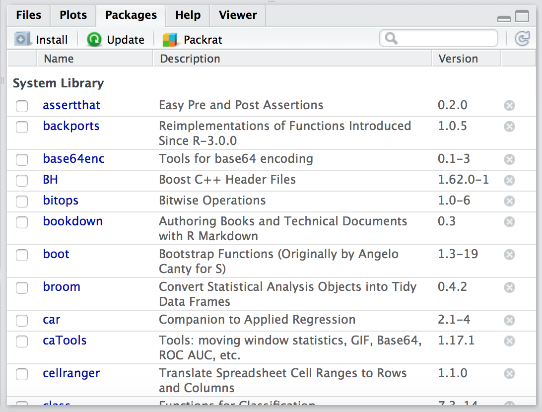
Figure 3.1: A screenshot of the packages tab in RStudio.

Next, select the install packages button:

Figure 3.2: The Install button in RStudio’s Packages pane.

This will bring up a dialog box similar to the one in Figure 3.3. The first drop down asks you from which R repository you would like to download a package. The default Repository(CRAN) will work well for our purposes. CRAN stands for the “Comprehensive R Archive Network” and it is usually easiest to download a package from one of the CRAN mirror sites. Ensure you are connected to the internet when installing packages. Next, enter the package name in the Packages field.

Enter: readr, ggplot2, psych

Keep the rest of the options as they appear by default. Then click the install button.

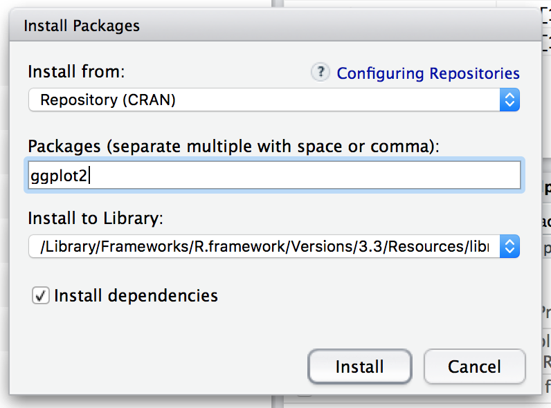
Figure 3.3: A screenshot of the install packages dialog box in RStudio.

Loading and unloading packages

To use an installed package in a session, load it with library(). Loading packages in code makes the script’s dependencies visible and reproducible. The checkboxes in RStudio’s Packages pane perform the same action interactively.

You could also type the command:

library(readr)
library(ggplot2)
library(psych)

In the future this will be useful when you are writing lines of R code that you want to reuse. It will be helpful to know which libraries are being used and called upon that are not loaded by default in RStudio.

Packages sometimes export functions or operators with the same name. R reports these masking messages when packages are loaded. When a name is ambiguous, identify the package explicitly with the namespace operator:

psych::describe(sidewalk)
ggplot2::ggplot(sidewalk)

This is clearer than repeatedly attaching and detaching packages. The matrix-multiplication operator in R is %*%; it is not %+%.

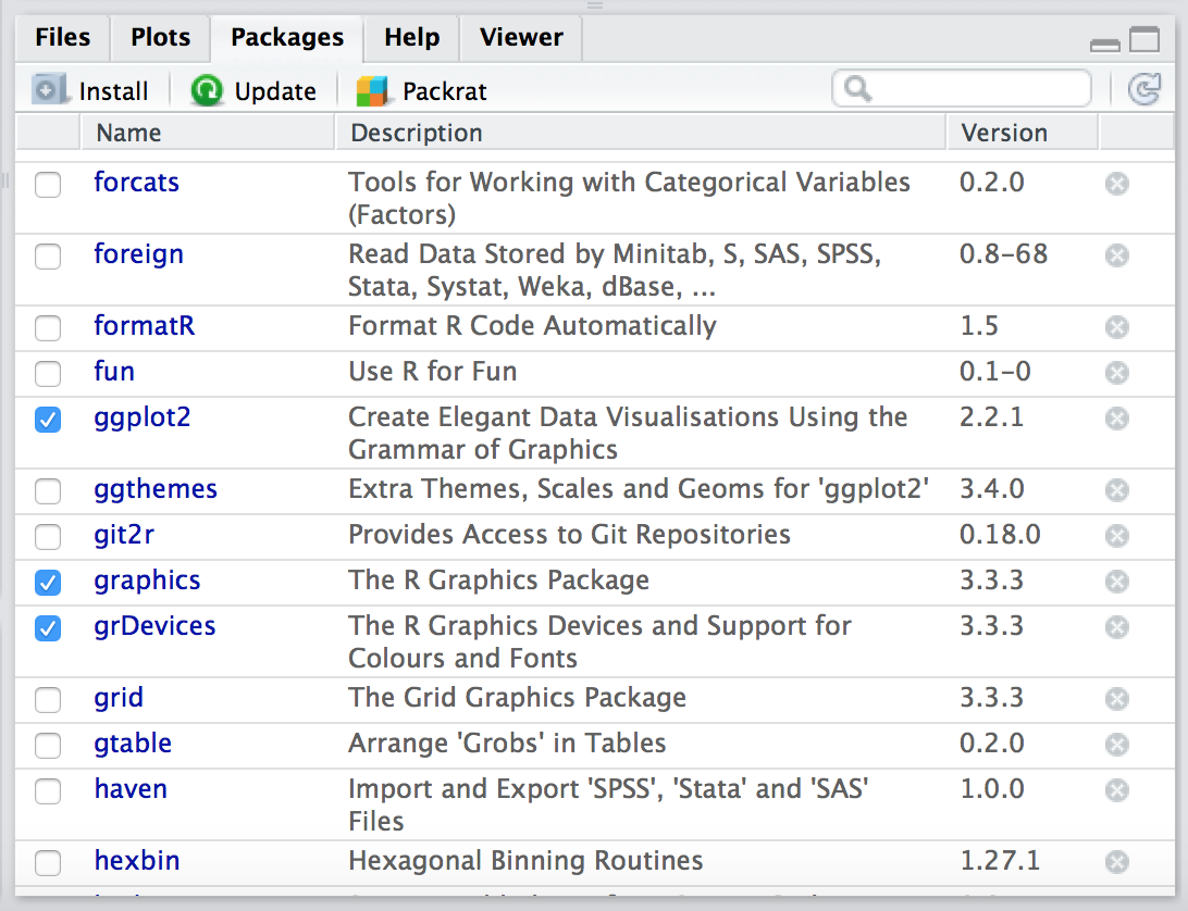
Figure 3.4: A screenshot of the packages tab in RStudio with packages selected.

Recommended packages

Other useful packages include tidyverse for data work and visualization, knitr for report generation, readxl for Excel files, and haven for SPSS, Stata, and SAS files. Install packages when a lesson requires them rather than installing an extensive list in advance.

Some recommended packages are not part of base R. For example, load readxl only when importing an Excel workbook:

library(readxl)

2. Organizing files with an RStudio Project

Keep the data, scripts, and reports for an analysis together. Create a dedicated folder for the project rather than scattering files across the Desktop or Downloads folder.

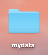
Figure 3.5: A dedicated folder for project files.

In RStudio, choose File → New Project → Existing Directory and select that folder. Opening the project sets the working directory automatically and makes relative paths such as "data/sales.csv" portable across computers.

RStudio also provides Session → Set Working Directory → Choose Directory, shown below. This changes the directory only for the current session and is less reproducible than opening a Project.

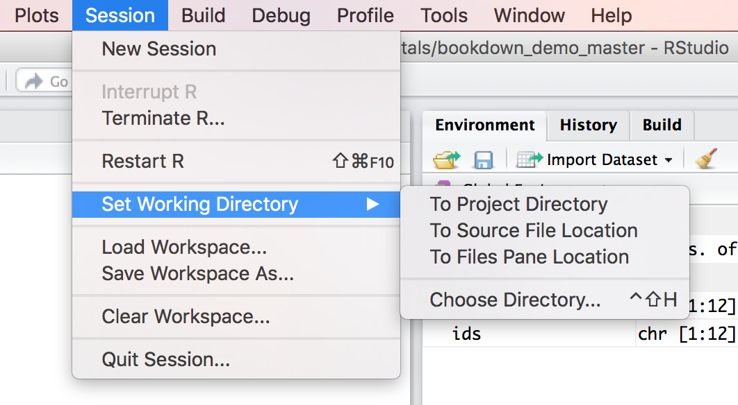
Figure 3.6: The Set Working Directory menu in RStudio.

You may encounter setwd() in older scripts. Avoid hard-coding a personal path in submitted work; prefer an RStudio Project and relative paths. Use getwd() to check the active project directory.

3. Downloading and importing data

R can import CSV, Excel, SPSS, Stata, SAS, and other formats. CSV is a portable choice for plain tabular data. Use readr::read_csv() for CSV files, readxl::read_excel() for Excel workbooks, and haven functions for common statistical-software formats.

Many course files use the .csv extension. CSV stands for comma-separated values: each line is a record, and commas normally separate its fields. CSV files store plain text and do not preserve spreadsheet formatting, formulas, or multiple worksheets.

Downloading Data

Before we can import a file, we need to have a file to import. Let’s use a file from NYC Open data on Sidewalk Cafes. You can download the dataset from https://becomingvisual.com/rfundamentals/Sidewalk_Cafes.csv

Find the Sidewalk_Cafes.csv file that you downloaded (you can probably find it in your Downloads folder on your computer) and move it to your mydata folder on your desktop.

Importing a dataset

Environment pane. In RStudio, the upper-right pane contains the Environment tab. Select Import Dataset to import a local CSV file interactively.

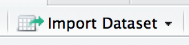
Figure 3.7: The Import Dataset control in RStudio’s Environment pane.

Select From Text (readr) to import a CSV file that is stored on your hard drive.

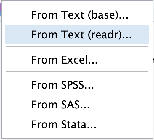
Figure 3.8: A screenshot of the Workspace in RStudio.

Next, navigate to the Sidewalk_Cafes file that you saved earlier by selecting the Browse button in the Import Text Data dialogue box shown below, see Figure 3.10.

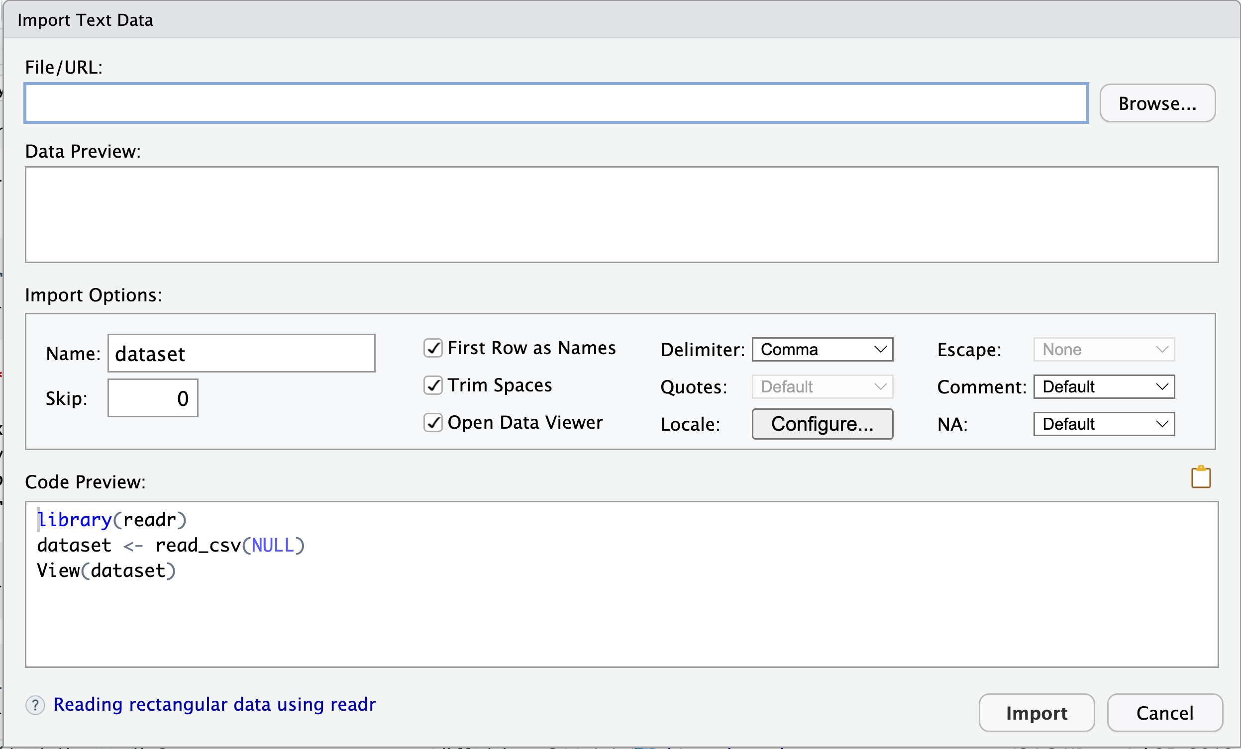
Figure 3.9: The RStudio Import Text Data dialog.

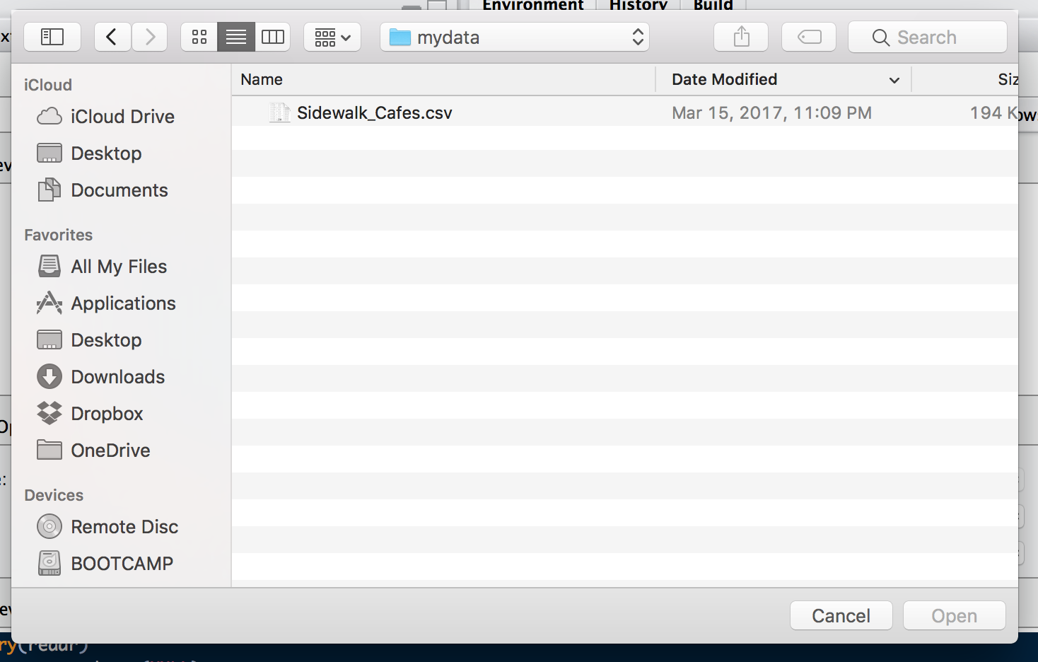
Figure 3.10: Navigating to your file in RStudio.

This will launch the Import Text Data window, see Figure 3.11. Here you can set your preferences for how you would like R to read in your .CSV file.

Name. First, you can name your dataset. There is already a default name given. Let’s replace it with sidewalk, as shown in Figure 3.11.

Heading. Select yes since the first row in the dataset contains the column headings. These include Entity.Type, License Number, Sidewalk.Cafe.Type., etc. If you do not select yes to heading, R will create a default header using V’s (e.g. V1, V2, V3). This works well if you do not have a header, but in our case we do and we don’t want R to create a header for us. If we selected no, our first row of data would contain the column names, such as Entity.Type, etc.

Delimiter. This is the character that separates fields in the CSV. In this case, the delimiter is a comma. You can see this in the input file window. Other options include whitespace, tab, or a semicolon.

Decimal. If there are decimal points in your data, select period to use the period character for the decimal point. This is the default setting and you can keep it set to period for our purposes. If needed, select comma to encode decimal points into commas.

Quote. If there are single quotes in your data, you can select to have them encoded as double quotes, single quotes, or none. You can keep the default setting.

Once you have set the import preferences, select Import. RStudio displays the generated read_csv() command; copy that command into your script so the import can be reproduced.

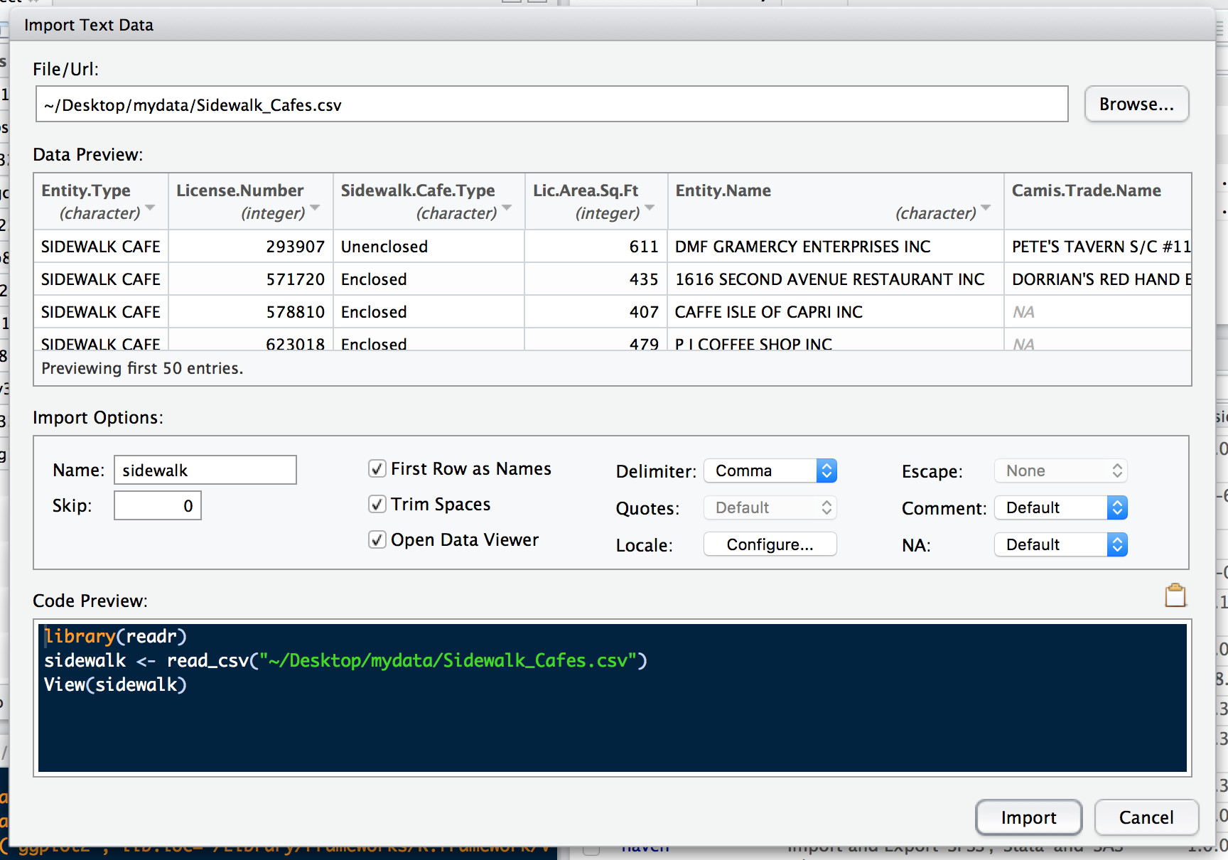
Figure 3.11: Setting import preferences in RStudio

Once you have imported the file, it opens in a Data Viewer tab in the Source pane, see Figure 3.12.

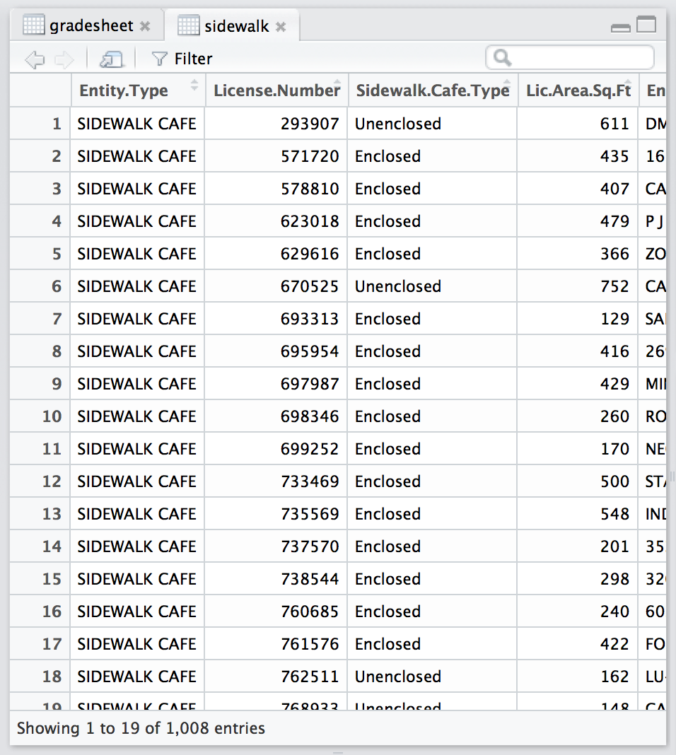
Figure 3.12: The sidewalk CSV file loaded in the source window.

The command to view the file in the source window is:

View(sidewalk)

The Data Viewer displays sidewalk in a spreadsheet-like view.

Check the object’s class with class().

class(sidewalk)

## [1] "spec_tbl_df" "tbl_df"      "tbl"         "data.frame"

The data contain rows (observations) and columns (variables). Use nrow() to count observations and ncol() to count variables.

nrow(sidewalk)

## [1] 1008

ncol(sidewalk)

## [1] 12

The row count is the number of observations in this copy of the dataset. The Data Viewer also displays the current numbers of rows and columns.

4. Working with missing data

Let’s do a little more with this data frame. Let’s say you wanted to know the average or the mean square footage for sidewalk cafes in NYC. Use the mean() function to compute this value for the variable Lic.Area.Sq.Ft.

mean(sidewalk$Lic.Area.Sq.Ft)

## [1] NA

However, you can see that R returns the value of NA. We were expecting a number, not NA. This is a clue that our data probably contains a special value, NA.

Let’s just view the sidewalk$Lic.Area.Sq.Ft variable.

View(sidewalk$Lic.Area.Sq.Ft)

If we scroll down in the source window (spreadsheet view) we can see there are some values of NA. The function mean( ) cannot compute the calculation because NA is not a number. Only numbers can be used to compute the mean. This is why the value of NA was returned from R.

Tell mean() to ignore missing values for this calculation by setting na.rm = TRUE. This does not delete rows or alter the original data frame.

mean(sidewalk$Lic.Area.Sq.Ft, na.rm = TRUE)

## [1] 258.6475

As you can see, we were able to compute the mean square footage for sidewalk cafes in NYC. About 259 square feet. We can use the round function that we learned earlier to round up from 258.6475 to 259.

round(mean(sidewalk$Lic.Area.Sq.Ft, na.rm = TRUE))

## [1] 259

At this point, you should practice retrieving variables and values from the sidewalk data frame. Return to session 2 to review working with data frames.

5. Extracting a subset of a data frame

Subsetting your data frame is useful if you want to select different variables within the data frame (i.e., keep only some of the columns) or a subset of observations (i.e., keep only some of the rows).

There are few ways to subset your data. I’ll introduce you to 3 simple ways.

Using the $ operator

If you only want to extract one column of your data frame you can use the $ operator. In the example below, we just called the column Address.Zip.Code from the sidewalk data frame and assigned it to a variable called zipcode. I just included a snippet of the values of zipcode. You can view a preview of the values by using the head function and specifying the number of rows to show.

zipcode <- sidewalk$Address.Zip.Code
head(zipcode, 5)

## [1] 10003 10028 10065 11201 10014

By default, our new variable zipcode is an integer since we assigned it a vector of numbers. If you need to change it to a data frame you can use the tibble() function from the tidyverse package as shown below.

class(zipcode)

## [1] "numeric"

zipcode <- tibble::tibble(zipcode)
class(zipcode)

## [1] "tbl_df"     "tbl"        "data.frame"

Using the subset( ) function

The subset( ) function is an easy way to select particular rows and columns. The function is organized as follows:

subset(x =, subset =, select =)

x. The data frame you want to subset

subset. A vector of logical values indicating which observations (rows) of the data frame you want to keep. By default all rows will be retained.

select. Indicates the variables (columns) you want to keep. By default all columns will be retained. Try to implement the example below. Here we are creating a variable sidewalk_subset to hold the data we are subsetting from sidewalk. In this example, we only want to keep those rows where the zip code is 10012. This is the zip code for NYU Stern. In addition, we want only the names of those locations (Entity.Name) to be returned.

sidewalk_subset <- subset(x = sidewalk, subset = Address.Zip.Code == 10012, select = Entity.Name)
sidewalk_subset

## # A tibble: 46 × 1
##    Entity.Name                       
##    <chr>                             
##  1 LU-ANN BAKERY SHOP INC            
##  2 CAFFE DANTE INC                   
##  3 CAVALLACCI, FABRIZIO              
##  4 DYNAMIC MUSIC CORP                
##  5 NILO INC.& VIOLA CONSULTING LLC   
##  6 FEENJON CORP                      
##  7 POMODORO RESTAURANT & PIZZERIA INC
##  8 DOJO RESTAURANT INC               
##  9 172 BLEECKER STREET RESTAURANT,INC
## 10 RESTAURANT VENTURES OF NY,INC.    
## # ℹ 36 more rows

Notice that the there is a number next to each observation or row. R automatically creates this. The numbers reference the given row from the data frame in which the data was extracted from (e.g. sidewalk).

Using square brackets

We can reference rows and columns of a data frame or vector using [ ]. The format for usage is as follows:

Data frame [rows, columns]

If we wanted the first 2 rows from sidewalk and 5th through 12th variables, Entity.Name through Location.1 we could write the following:

sidewalk[1:2, 5:12]

The colon represents a range. The ranges here are 1:2 (rows 1 through 2) and 5:12 (columns 5 through 12). However, there are times when you want to reference rows and columns that are out of a range sequence. For example, let’s say you wanted to extract rows 1 through 100 for only columns 3 and 5. To do this you need to use the combine function for your rows and columns values.

sidewalk[c(1:100),c(3,5)]

If using numbers for variable (column) names (e.g. 3, 5) become too abstract, you can always pass in the actual name of the column. See the example below.

sidewalk[1:100, c("Sidewalk.Cafe.Type", "Entity.Name")]

Moreover, there are times where you want to display all the rows or all of the columns. This can be done by simply leaving the row or column value blank (but keep the comma to separate the row and column parameters). See below for an example that displays all the rows, but only two columns.

sidewalk[, c("Sidewalk.Cafe.Type", "Entity.Name")]

The example below displays all columns, but only the first 100 rows.

sidewalk[1:100, ]

Finally, you may want to find where a particular value is located in the data frame by the index number (row number). This can be done using the which() function.

For example, you may want to know which rows have sidewalk cafes in the Lower East Side with the zip code equal to 10009.

which(sidewalk$Address.Zip.Code == 10009)

##  [1]  33  46 129 205 216 228 234 249 258 322 374 510 519 573 614 629 670 696 713
## [20] 752 771 788 806 813 860 893 956

This returns those row numbers that you can use pass in to the sidewalk data frame to return back only specific rows.

sidewalk[which(sidewalk$Address.Zip.Code == 10009), ]

## # A tibble: 27 × 12
##    Entity.Type   License.Number Sidewalk.Cafe.Type Lic.Area.Sq.Ft Entity.Name   
##    <chr>                  <dbl> <chr>                       <dbl> <chr>         
##  1 SIDEWALK CAFE         811344 Unenclosed                    251 SEVEN A CAFE …
##  2 SIDEWALK CAFE         853927 Unenclosed                    443 THREE BEANS I…
##  3 SIDEWALK CAFE         960517 Unenclosed                     61 NERA CORP.    
##  4 SIDEWALK CAFE        1034831 Unenclosed                    501 177 CHRYSTIE …
##  5 SIDEWALK CAFE        1066226 Enclosed                       NA L & L FOODS O…
##  6 SIDEWALK CAFE        1073840 Unenclosed                    178 ITALIAN MOTHE…
##  7 SIDEWALK CAFE        1076706 Unenclosed                    482 EAE, CORP     
##  8 SIDEWALK CAFE        1097153 Unenclosed                    162 RAGUBOY CORP. 
##  9 SIDEWALK CAFE        1102989 Unenclosed                    532 ZUMSCHNEIDER …
## 10 SIDEWALK CAFE        1142739 Unenclosed                    192 LGR FIRST CORP
## # ℹ 17 more rows
## # ℹ 7 more variables: Camis.Trade.Name <chr>, Address.Street.Name <chr>,
## #   Street.Address <chr>, Address.Location <chr>, Address.Zip.Code <dbl>,
## #   Camis.Phone.Number <dbl>, Location.1 <chr>

6. Working efficiently with R scripts

Chapter 1 introduced R scripts as the saved record of your work. This section develops a more efficient script workflow for an analysis that uses packages, external data, multiple processing steps, and reusable output.

A well-organized script should run from top to bottom in a fresh R session. Its package calls, file paths, transformations, and output should appear in a logical order. Advantages include:

You preserve and reproduce the analysis.
You can reuse and revise code.
You can document assumptions and decisions.
You can share the workflow with collaborators.
You can run a complete sequence instead of rebuilding it in the Console.

Create a script with File → New File → R Script. Save it as sidewalk.R inside the current RStudio Project. The script opens in the Source pane (Figure 3.13).

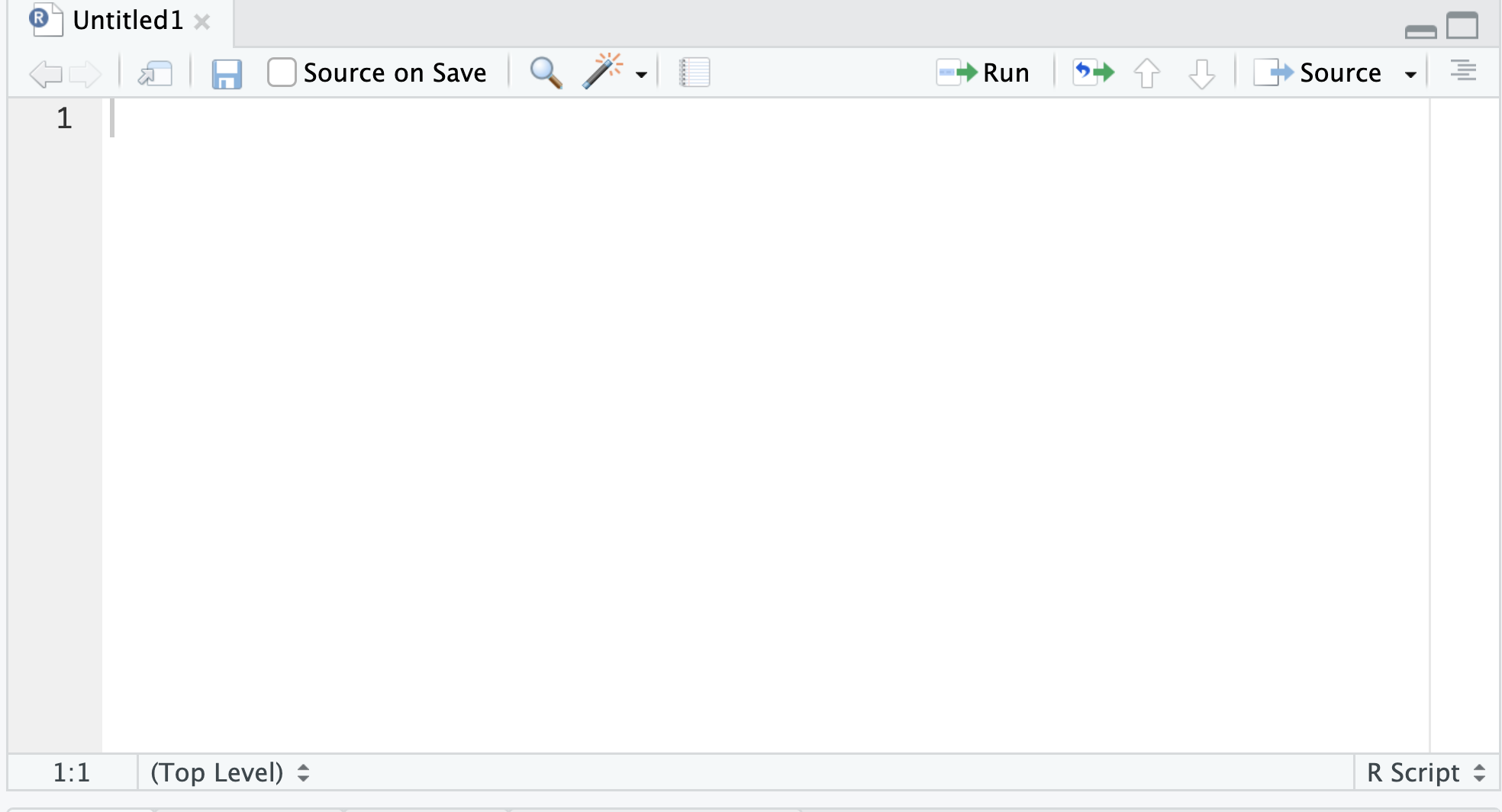
Figure 3.13: A new R script file shown in the source panel in RStudio.

In your R script, you’ll notice the number 1. This indicates line 1 in the file. You can begin typing your R commands in this file. Type the commands you see in Figure 3.14. Then save your file by going to File > Save.

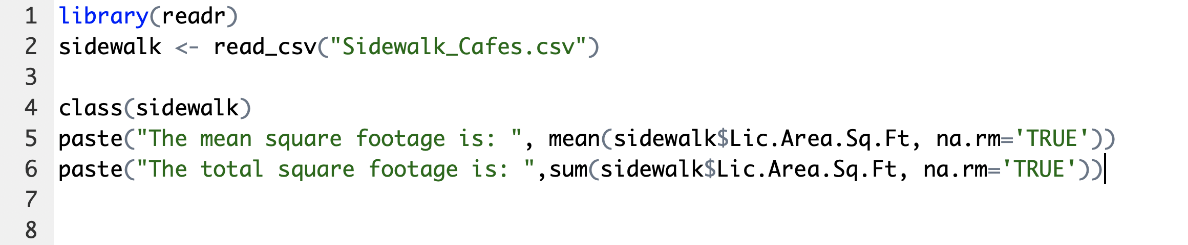
Figure 3.14: R commands written in an R script file.

The script should begin with required package calls and data import, followed by inspection, transformation, analysis, and output. In the example, sum() adds the values in Lic.Area.Sq.Ft; na.rm = TRUE tells the function to ignore missing values for that calculation.

Note: These commands will not be executed until you actually run the script.

Running R scripts

There are several ways to run code from an R script.

Option 1. To run a saved script from the project directory, use:

source("sidewalk.R")

However, this method requires you to be very explicit about printing out values to the console. If you run the command above, you’ll notice the sum and mean were not printed. You would have to modify your file to include the print() function. See lines 5 and 6 in the script below.

Figure 3.15: The addition of the print command to enable printing in the console from an R script that is executed using the source( ) function.

You’ll notice that we are calling a function within a function. We are passing the output of the sum() function to the print() function. See below for the output in the console.

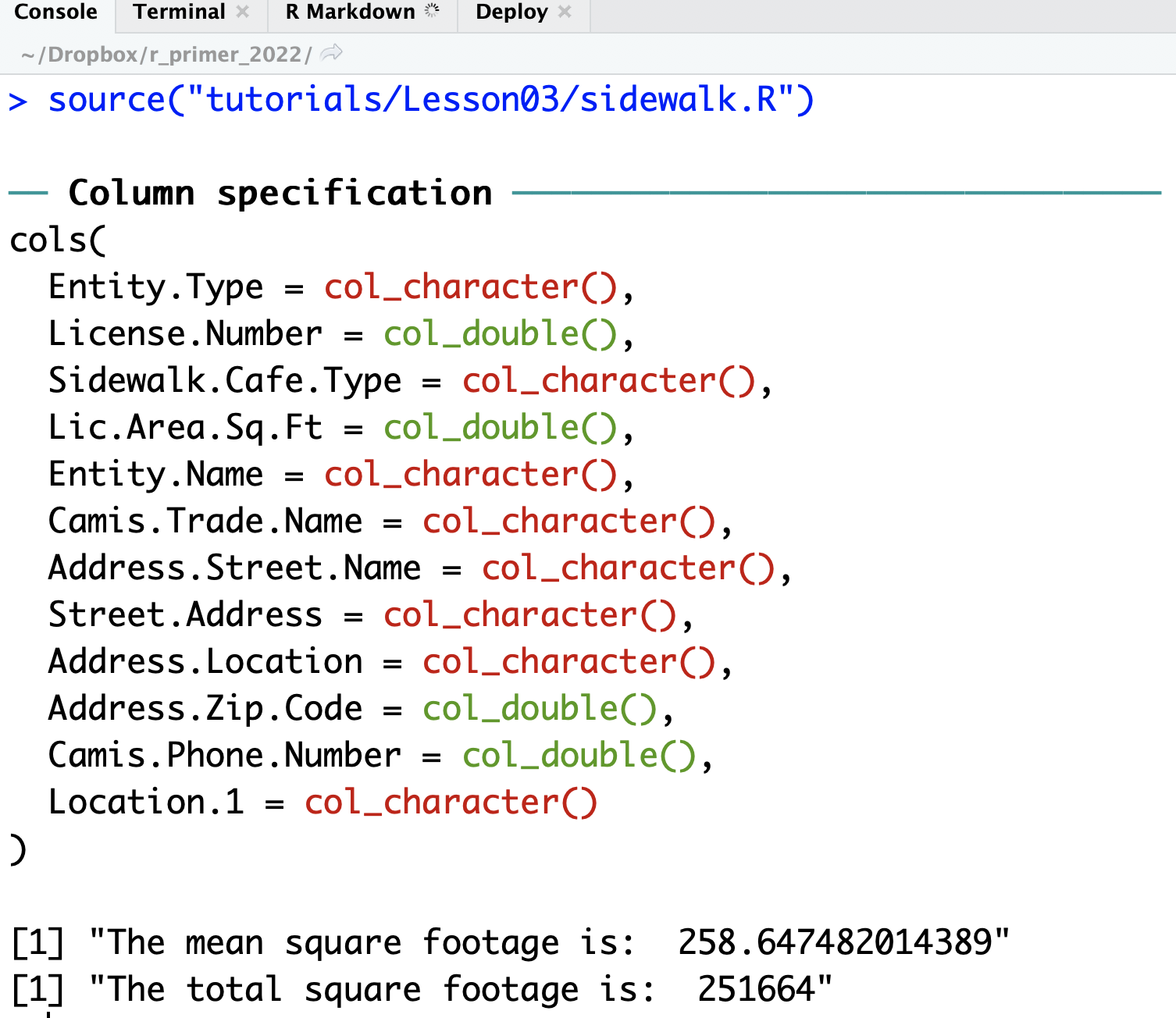
Figure 3.16: The addition of the print command to enable printing in the console from an R script that is executed using the source( ) function.

Option 2. Run the current line or selected code from the Source pane by clicking Run or pressing Ctrl+Enter on Windows/Linux or Command+Enter on macOS.

Figure 3.17: The Run control in the RStudio Source pane.

To run several lines, select them and use the same command. To source the entire saved script, click Source. Try it.

For the rest of this course, use R scripts and R Markdown documents as the durable record of your work. The Console remains useful for quick experiments.

7. Adding comments and documentation

Comments explain intent, assumptions, and important decisions. Useful comments help collaborators—and your future self—understand why the analysis was performed, not merely restate what an obvious line of code does. See Figure 3.18 for an example.

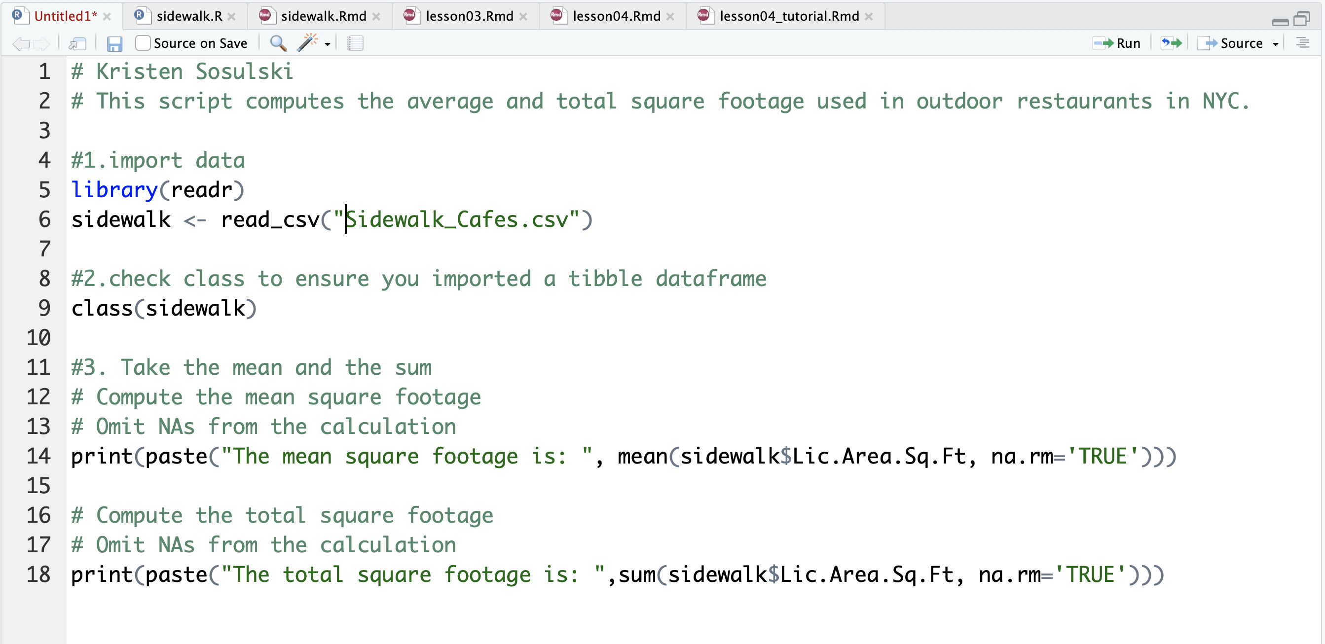
Figure 3.18: Comments added to the existing RScript file.

The comment character, # tells R to ignore everything written to the right of the #. We use the # for each line we would use for commenting our code. In RStudio, the color of the text will change to indicate that you are writing a comment. Syntax colors depend on the selected RStudio theme, but comments will appear visually distinct from executable code.

Try it. Create a script with comments similar to Figure 3.18.

To execute this script, highlight the text and click the run button.

Figure 3.19: The Run control used to execute selected R code.

8. Creating reports

Suppose a weekly sales file arrives in the same format. A reproducible report can rerun the calculations and visualizations when the data change. knitr executes R code embedded in a document, and R Markdown can render the combined narrative, code, and results to HTML, Word, or PDF.

PDF output requires a LaTeX distribution. TinyTeX is a convenient option for R users. HTML and Word output do not require LaTeX.

To create dynamic reports, follow along with the instructions below.

a. Install knitr

Begin by installing the knitr package along with any identified dependencies in RStudio.

b. Modify your RScript

Working with your sidewalk.R add a simple box plot using the code on line 21.

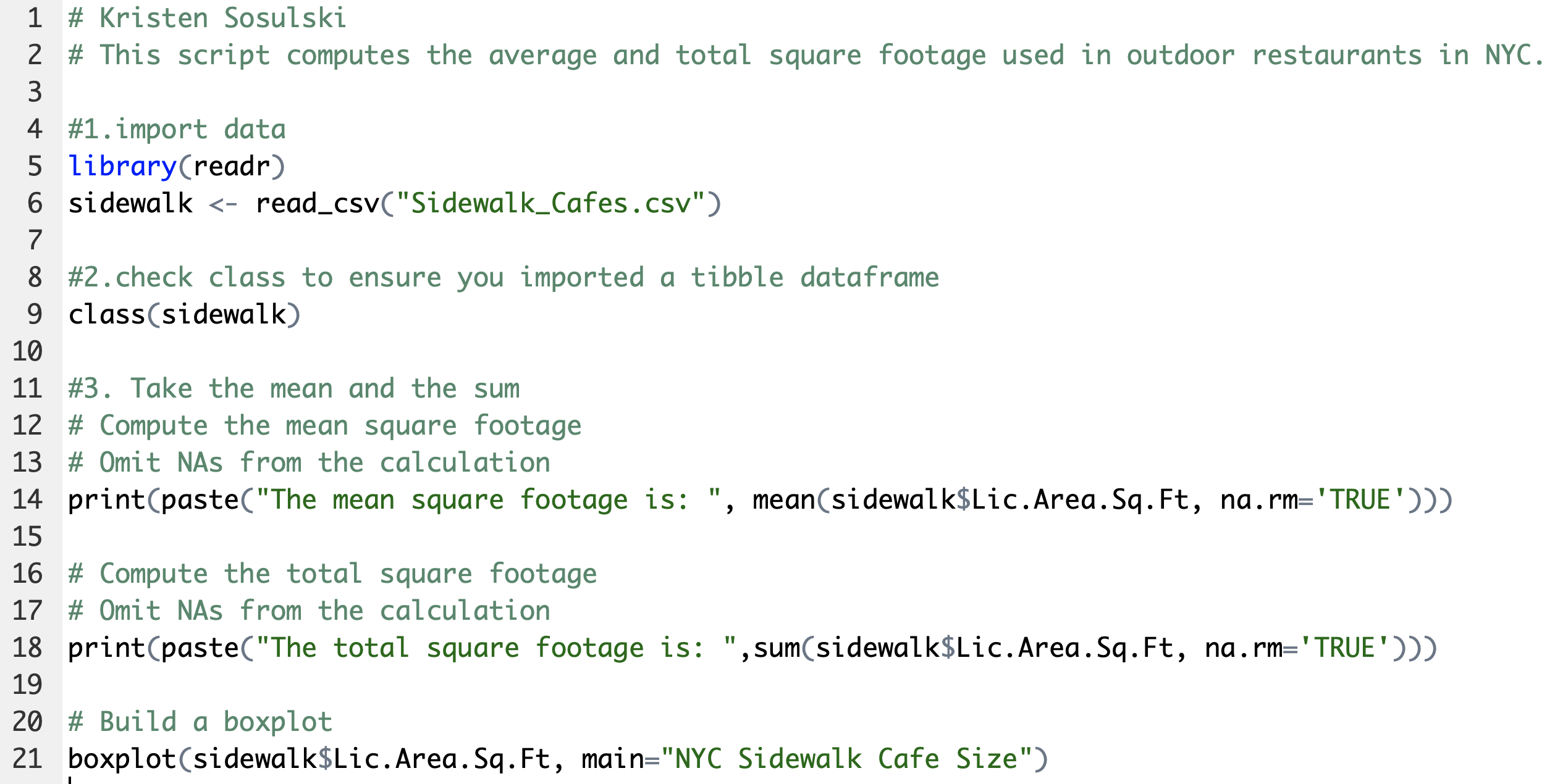
Figure 3.20: The sidewalk example 01.R file

c. Create an MS Word document from your R script

Click on the “Compile Report” button. You can also chose the “Compile Report” command from the File menu.

Figure 3.21: The Compile Report control for an R script.

Choose an output format: HTML, Word, or PDF. PDF output requires LaTeX; for this activity, choose Word.

Below, is the compiled notebook from the RScript. This format makes it easy to add explanatory notes. The plot is also created and included. Notice that the output of each command is denoted with ## interspersed with the R code. That is helpful since any line that begins with # is treated as a comment. So anyone who wants to run the code can copy and paste then entire block of text, including the output into the console, and it the code will be executed, but the old output will be ignored.

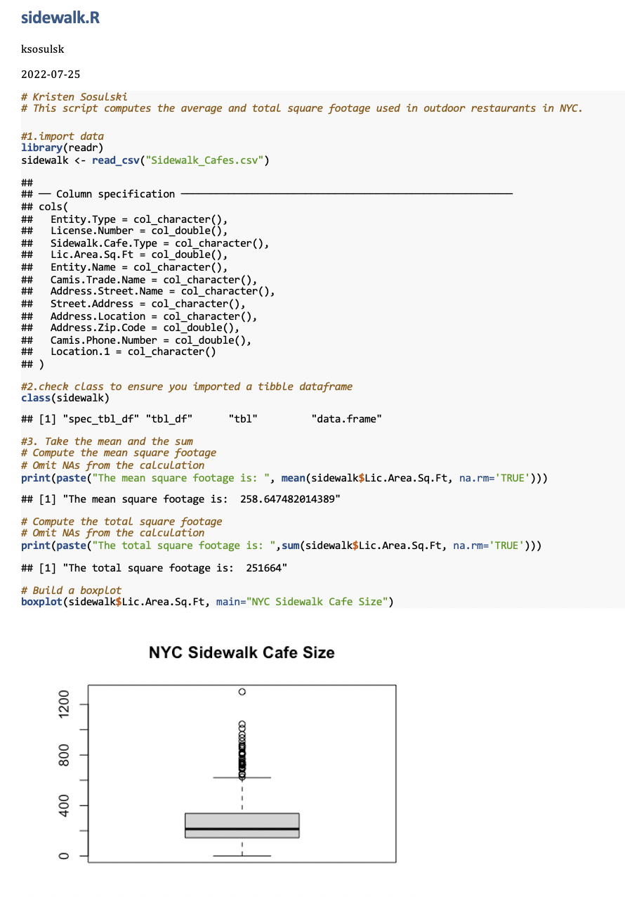
Figure 3.22: R Script compiled as a MS Word document

d. Creating an R Markdown File

The above example demonstrated how to publish your R script in a readable format, but it still has some drawbacks. Suppose you want to create a report that updates automatically? The above method will still be easier than manually creating the report each time, but formatting and adding comments will still have to be done manually every time the report is run. An R Markdown file combines narrative, R code, and output so that data preparation, analysis, and report generation can be reproduced.

Try it – A short activity

To get started go to the File menu, click New File > R Markdown as shown in Figure 3.23.

(Note: The first time you do this you may be prompted to install several packages.)

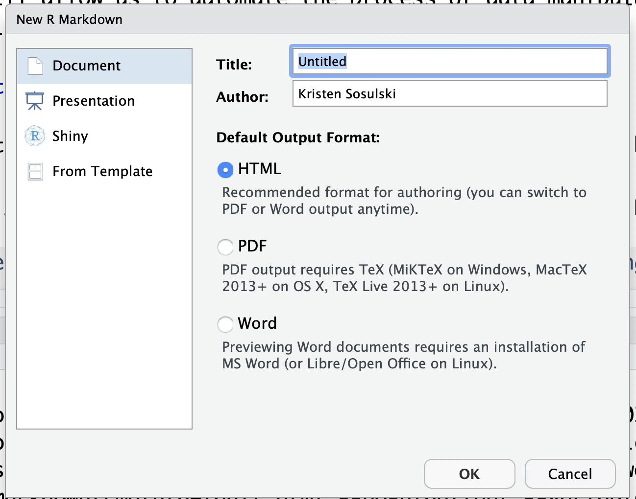
Figure 3.23: The dialogue box prompt for creating a new R Markdown document.

Title and Author: Enter a name for the file, and your name. Select HTML as the default output format. Click OK.

RStudio creates an .Rmd file containing a YAML header, narrative text, and executable R code chunks. It can be rendered to HTML, Word, or PDF. RStudio also supports Quarto (.qmd), but this course continues to use R Markdown because the website is built with Bookdown.

The following is the example Markdown file:

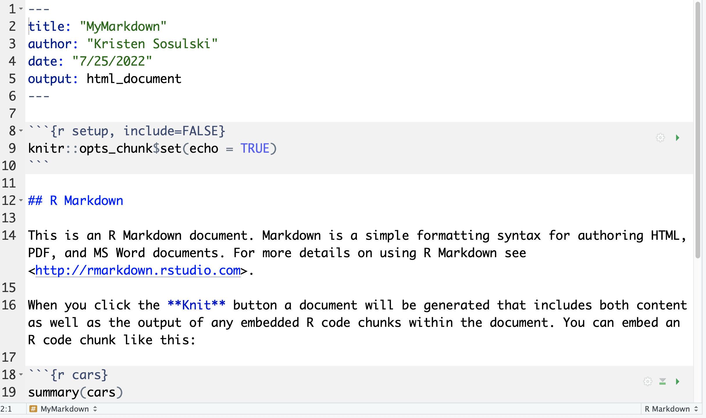
Figure 3.24: A sample Markdown file.

To see the HTML file, select

Figure 3.25: The Knit control for rendering an R Markdown document.

The output is shown in Figure 3.26 below.

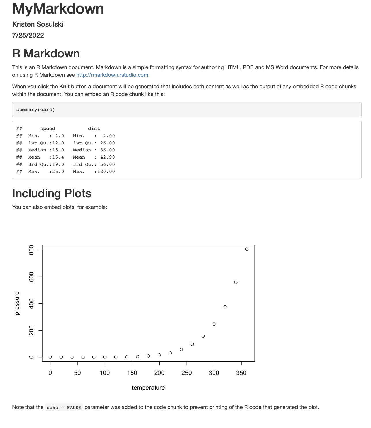
Figure 3.26: The R Markdown HTML document.

Some Basic R Markdown Syntax

Markdown is a lightweight syntax for structuring plain text. R Markdown extends it by allowing R code and its output to be embedded in the document.

Markdown syntax identifies headings, emphasis, lists, and other document elements. R code is embedded in chunks. Set echo=FALSE to run a chunk without displaying its source code, or eval=FALSE to display code without running it.

Document Heading
---
heading text
---

Bold
**text**

Italic
*text*   

List
* Item 1
* Item 2
    + Item 2a
    + Item 2b

R Code

\`\`\`{r}
place the R code here
\`\`\`

R Code With Options

\`\`\`{r echo=FALSE}
# Place R code here
\`\`\`

Set `echo=FALSE` to show a chunk's results without displaying its source code. Set `eval=FALSE` to display code without running it.

Inline R Code

You can place R code in the middle of a sentence using &#96;r expression&#96;.

For additional options, consult R Markdown: The Definitive Guide and the knitr chunk-options reference.

An R Markdown Example

Let’s say that New York City wants to track the square footage trend of enclosed versus unenclosed sidewalk cafes. They want a webpage that will show everyone the current distribution of square footage of enclosed versus unenclosed sidewalk cafes, as well as some of the code that was used to perform the calculations. We’ll create the entire report using an R Markdown file.

Start off with the Markdown file we opened earlier. Delete everything except the title block, which you can modify to your liking, see Figure 3.27. Below the three dashes that end the title block is where we add our text. Let’s put in a quick line of introduction, for that we can use plaintext. It may be a good idea to show when the report was generated, so we can use the inline R code call discussed above to add the date. Inline code such as 2026-08-28 inserts the rendering date. Let’s add that to our introductory text. See below:

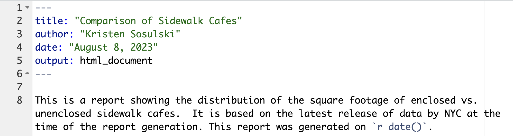
Figure 3.27: A markdown document in R.

To generate your HTML, Word, or PDF file, you just click on the Knit button that you see in the above image. Below is the generated report. Notice the date of the execution has been placed in the report. The inline code execution option can be particularly useful for placing summary statistics into the narrative description.

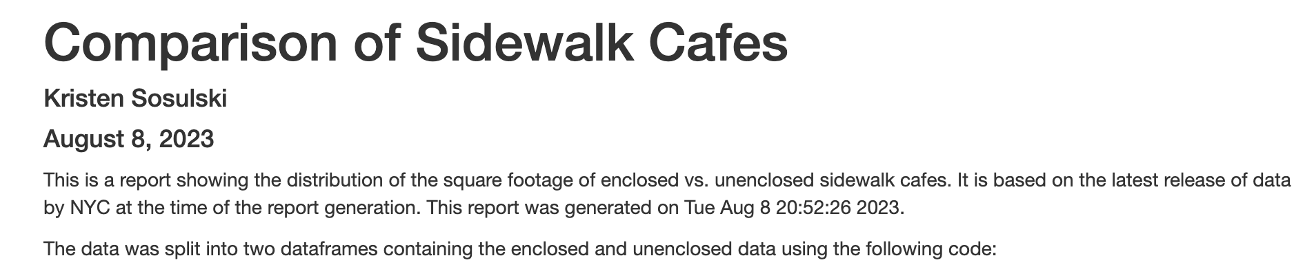
Figure 3.28: The HTML output of the R markdown file.

The next step is to import the sidewalk cafe data. Since this is a trivial step for this report we will not include or “echo” this code into the report.

You can begin by inserting an R code block or chunk into the Markdown file, using the syntax given in the previous section.

You could also use chunks with the Insert button to save some typing.

Figure 3.29: The Insert control for adding an R code chunk.

Inside the code chunk, type the command to import the data. You can test your R code execution from the drop down menu on the Chunks button. You can see the results of executing the code chunk in Figure 3.28. The import command was executed, and the sidewalk data frame is now created.

Figure 3.30: A code chunk highlighted in RStudio.

Now we have to process the data, specifically we want to split the sidewalk café data set into two sets, representing the enclosed and unenclosed data. This code is a little more complex, so perhaps we want to add a line or two of explanation before this step. You can see the narrative for the report, and the second code chunk in the screenshot of the Markdown file below.

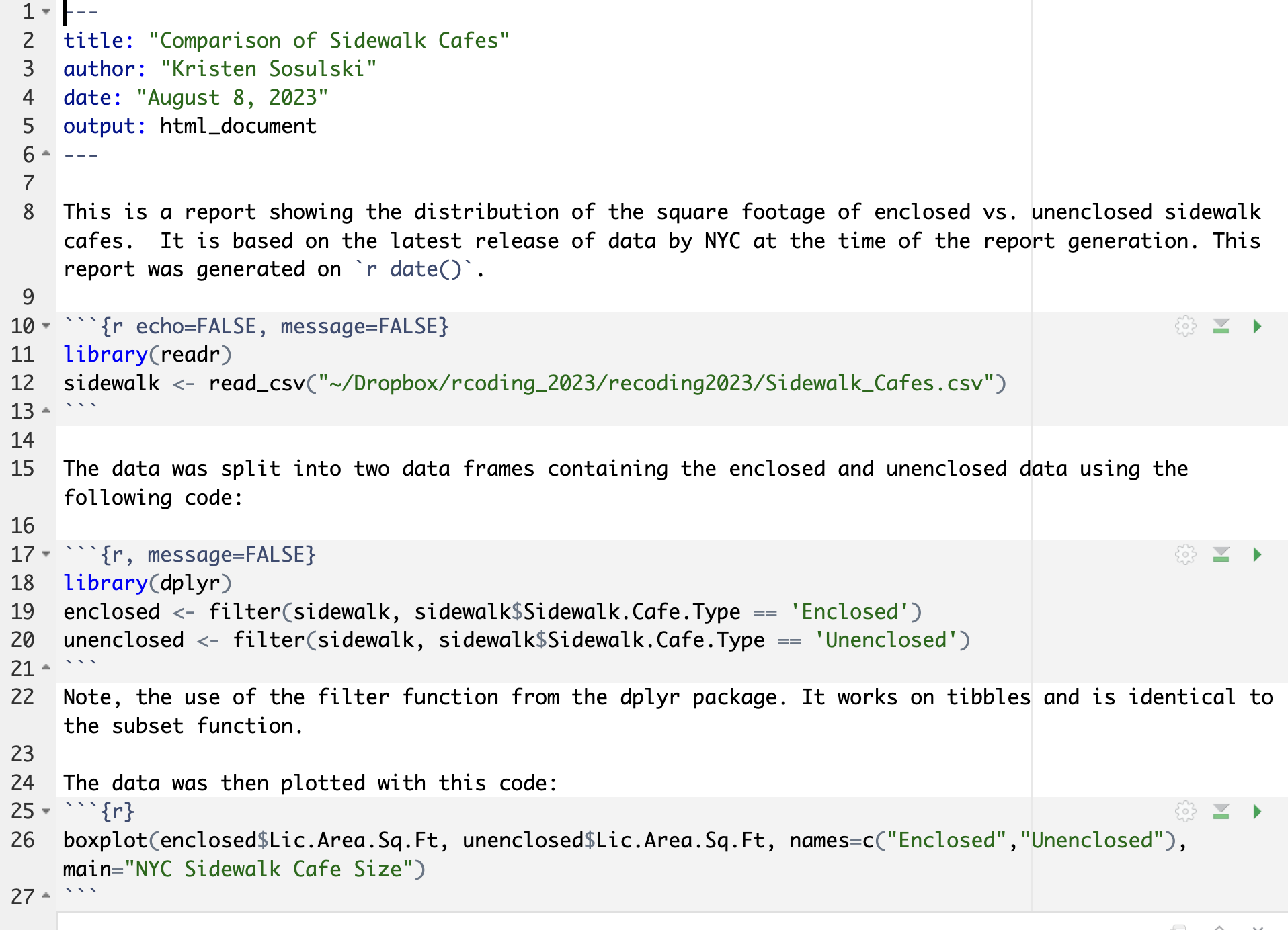
Figure 3.31: A second R code chunk in the sidewalk-café report.

And below is the additional portion of the report. Remember, we echoed back the code this time. Since filtering (or subsetting) the data frame doesn’t produce any visual output, there is no evaluation of the code to add to the report, but the code is executed nonetheless.

The data was split into two data frames containing the enclosed and unenclosed data using the following code.

library(dplyr) enclosed <- dplyr::filter(sidewalk, Sidewalk.Cafe.Type == "Enclosed")

unenclosed <- dplyr::filter(sidewalk, Sidewalk.Cafe.Type == "Unenclosed")

The final step for this report is to produce the box plot. Again, we will insert some descriptive narrative, and show the code used to produce the plot. However, since this time there is output from the execution of the R code, the visualization will also be added to the report. The final report, encompassing the entire Markdown file, is shown on the next page.

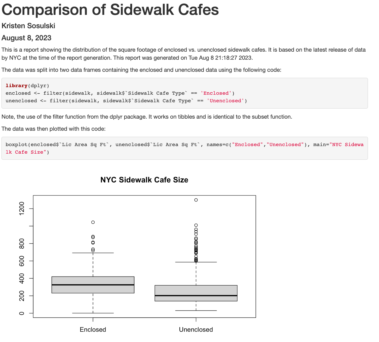
Figure 3.32: The completed R Markdown source document.

Publishing to RPubs

You can publish rendered HTML documents to RPubs. RPubs pages are publicly accessible: never publish confidential company, client, employee, or student data. After you run Knit HTML, you will see an option to publish. Select, Publish and the RPubs dialog box will appear. Select Publish. Next, choose RPubs.

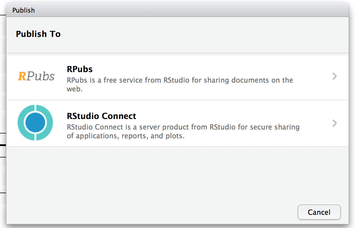
Figure 3.33: The Publish control displayed after rendering an HTML document.

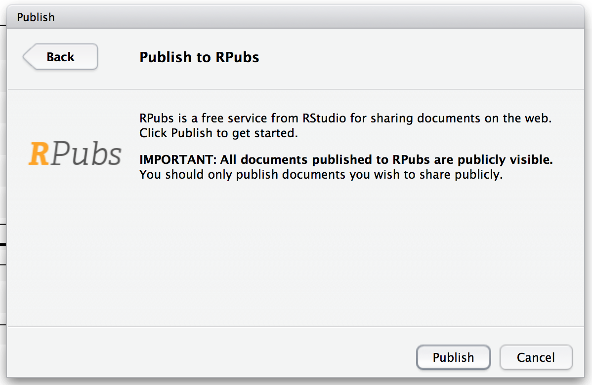
Figure 3.34: Selecting RPubs as the publishing destination.

You will be prompted to sign in to RPubs or create an account.

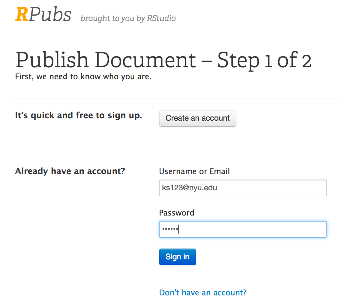
Figure 3.35: The RPubs sign-in screen.

After you create an account, provide your document with a title.

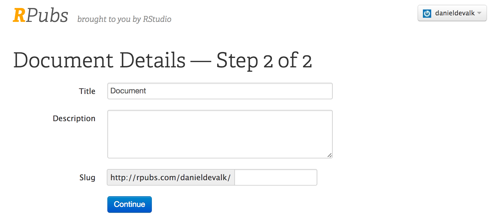
Figure 3.36: Entering a title before publishing an RPubs document.

Then you will be provided with a URL you can share and update. The published document is below and available at: https://rpubs.com/sosulski/1070147

This section introduced the knitr package and R Markdown, and demonstrated some of the basic functionality. There is much more functionality than was demonstrated here, for example Markdown can also easily add tables to reports and there are many additional formatting options. There are other modules, Shiny, for instance, that can be used to add interactivity.

9. Summary

This lesson moved your work from one-off Console commands to a reproducible project. You learned to:

install a package once and load it when a script needs it;
use explicit namespace calls such as readr::read_csv() when helpful;
organize files in an RStudio Project and use relative paths;
inspect the rows, columns, names, and structure of imported data;
handle missing values deliberately with arguments such as na.rm = TRUE;
select rows and columns with $, subset(), or square brackets;
save reusable commands in an R script and document important decisions with comments;
render narrative, code, and results from R Markdown; and
publish only data and reports that are appropriate for public access.

Useful commands include installed.packages(), library(), readr::read_csv(), nrow(), ncol(), names(), str(), mean(), sum(), source(), and print().

3.1 Exercise 3.1

We will be using basketball data from March Madness for this exercise.

Data

Download from: March Madness CSV

Data Dictionary

Variable	Description
Rank	Team Ranking
Previous	Previous Team Ranking
School	Name of the College or University
Conference	NCAA Conference (30 +)
Record	Overall Record
Neutral	Record with games in a neutral location
Home	Record with games at home
Non Div I	Record with non-divison 1 games

Write a R script to do the following:
(Remember to add comments)

Open the course RStudio Project and confirm the project directory with getwd().
Import the CSV file with readr::read_csv() using a relative path.
view the file
print number of rows and columns – Hint: dim()
print columns names
change column names to lower case so it is easier to use Hint: names(df_name) <- tolower(names(df_name))
explore the variable types. – Hint: str()
how many different conferences are there?
Let’s look at the difference in values of first two columns:

compute a new vector called “diff” and calculate the difference in rank and previous
print count and list of schools that changed 3 or more places Hint: create subset that satisfies criteria

3.1.1 Code walkthrough

3.2 Exercise 3.2

Tips:

Import the package readr to use the read_csv() function
When selecting the column for each year, use double quotes (or back ticks) around the number. For example, use gdp$"2017".

1a. Import the GDP dataset

1b. Compute the difference in GDP between 2007 and 2017 for each country. Download the GDP CSV.

Task:

Create a subset of countries that saw an increase of over one trillion dollars.

3.2.1 Code Walkthrough

3.3 Assignment 3a

The exercise described below will prepare you to work with external datasets in R. We will be working with the data on the usage of stimulus/recovery funds provided through the American Recovery and Reinvestment Act of 2009 (ARRA) from NYC Open Data. Please complete this exercise prior to moving on to the next lesson. Follow the instructions below. Submit a Word version or PDF of your R Markdown (with input and output shown) for this assignment.

Create a new R Markdown in RStudio named fed_stimulus.Rmd. Include your name and date
Go to NYC Open Data and export the Federal Stimulus dataset as a CSV file from https://data.cityofnewyork.us/Business/Federal-Stimulus-Data/ivix-m77e
Review the details of the variables included in the dataset by selecting the about section on the NYC Open Data website for the Federal Stimulus data.
Rename the downloaded file to Federal_Stimulus_Data.csv and save it inside the course project folder.
Write the code in your Rmarkdown to import Federal_Stimulus_Data.csv. Change the name of the data frame from Federal_Stimulus_Data to fed_stimulus
Compute the sum and mean for the payment value column
Create a subset of your data that returns those projects with project status is equal to the completed 50% or more. Do not include fully completed projects.
Review the analysis and add concise explanatory comments and narrative.
Knit the R Markdown document to Word or PDF. Confirm that the requested code and relevant output are included.

3.4 Assignment 3b

Answer the following questions using an R Markdown document

Download the S&P 500 historical prices from January 1st, 2022 to January 1st, 2023 as a spreadsheet from the Wall Street Journal: https://www.wsj.com/market-data/quotes/index/SPX/historical-prices

Create a new R Markdown file. Install quantmod if necessary, then load it in a setup chunk. Use chunk options to suppress package startup messages and warnings where appropriate.
Import the data file. Include the code. Use the R Chunk options to suppress warnings and messages.
Clean the data by checking for missing values and removing any rows with missing values. Store the result in a new data frame called clean_sp500_data. Show both the code and the output using the appropriate R Chunk options.
Subset the Date and Close columns from the data frame to a new data frame named historical_prices. Show both the code and the output using the appropriate R Chunk options.
Use the getSymbols() function from the quantmod package to download the daily stock prices for Wells Fargo (WFC) from January 1st, 2022 to January 1st, 2023. Store the data in a variable called wfc. Show both the code and the output using the appropriate R Chunk options.

Below is the code to return the daily stock prices for WFC.

wfc <- quantmod::getSymbols("WFC", from = "2022-01-01", to = "2023-01-01", auto.assign = FALSE)

Preview the first five rows with head(wfc, 5). Show the code and output.
Extract the Close column from the data frame and save to a variable. Show both the code and the output using the appropriate R Chunk options
Calculate the daily returns for WFC and store the result in a variable called wfc_returns. Show both the code and the output using the appropriate R Chunk options
Use comments for code-level decisions and R Markdown narrative to explain how each question is answered.
Render your .Rmd file as a Word Document.